Building a Distributed GBM on H2O

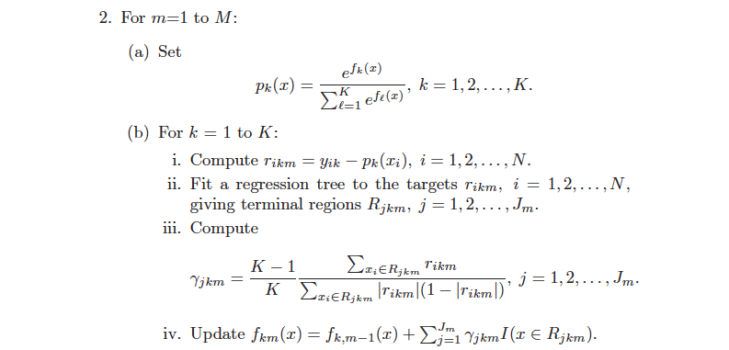
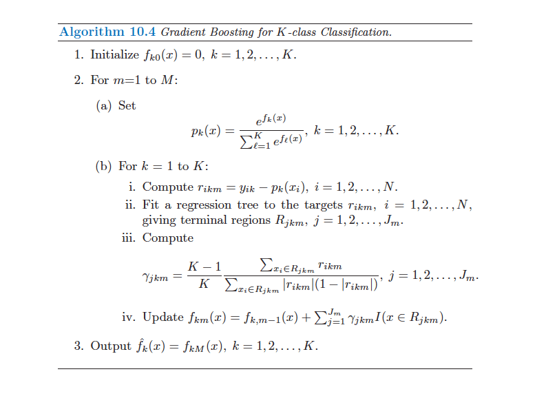
At 0xdata we build state-of-the-art distributed algorithms – and recently we embarked on building GBM , and algorithm notorious for being impossible to parallelize much less distribute. We built the algorithm shown in Elements of Statistical Learning II , Trevor Hastie, Robert Tibshirani, and Jerome Friedman on page 387 (shown at the bottom of this post). Most of the algorithm is straightforward “small” math, but step 2.b.ii says “Fit a regression tree to the targets….”, i.e. fit a regression tree in the middle of the inner loop, for targets that change with each outer loop. This is where we decided to distribute/parallelize.
The platform we build on is H2O, and as talked about in the prior blog has an API focused on doing big parallel vector operations – and for GBM (and also Random Forest ) we need to do big parallel tree operations. But not really any tree operation; GBM (and RF) constantly build trees – and the work is always at the leaves of a tree, and is about finding the next best split point for the subset of training data that falls into a particular leaf.
The code can be found on our git:
http://0xdata.github.io/h2o/
For GBM, look in:
src/main/java/hex/gbm/GBM.java - driver, main loop from ESL2
src/main/java/hex/gbm/SharedTreeBuilder.java - shared with RF, score & build 1 layer
src/main/java/hex/gbm/DBinHistogram.java - collect & split histograms per leaf
The High Level Bits
We do a straightforward mapping from vectors to leaves of a tree: we assign a “leaf id” or “node id” to each data row in a new temp vector. We also choose split points (based on the last pass) before making a pass over the data –
split-point decisions are made on summaries from the previous pass and are always “small data”, and typically aren’t useful to parallelize. Splitting a leaf makes it an internal node, and we add 2 new leaves below it.
On each pass through the data, each observation R starts at an internal tree node; we get the node id (nid) from our temp vector. The nid is a direct mapping into a POJO (Plain Old Java Object) for that node in a tree. The node contains the split decision (e.g., “if age<45 go left, else go right”). We move the observation R down the decision tree, left or right as appropriate, into a new leaf and record the new nid for next pass in our temp vector.
We then accumulate enough stats to make split decisions for the new leaves at the end of this pass. Since this is a regression tree, we collect a histogram for each column – the mean & variance (using the recursive-mean technique). Later we’ll pick the split point with the least variance, and the prediction if we don’t split will be the computed mean.
We repeat this process of moving a row R left or right, assigning a new nid, and summing into the histogram, for all rows. At the end of this pass we can split each current leaf of the tree, effectively building the tree one layer in a breadth-first fashion. We repeat for each layer, and after one tree is built we start in on the next.
Effectively then, we’re entirely parallel & distributed within a single tree level but not across trees (GBM trees have sequential dependencies) nor within levels of the same tree. This parallel-within-level aspect means there’s an upper bound on tree building speed: the latency to build a single level. However, since we’re completely parallel within a level we can make a single level faster with more CPUs (or conversely build a tree with more data in the same time). In practice, we’re the fastest single-node GBM we’ve ever seen and we can usefully scale-out with datasets as small as a few 10’s of megs.
Binning
Finding an optimal split point is done by choosing a column/predictor/feature and a identifying the value within that feature to be the point at which the data are split so as to minimize some loss function such as Mean Squared Error (or maximize information gain). The problem devolves to finding the optimal split value for a particular feature (and taking the max across all features). The optimal split is often found (with small data) by sorting the feature values and inspecting the induced split. For big data, this can be a problem (e.g. a distributed sort required for each tree leaf). We choose to approximate sorting with binning instead.
Binning (i.e. a radix sort) is fast & simple, can be done in the same pass as our other tree work, and can get arbitrarily close to the sorted solution with enough bins. However, there’s always the question of unequal binning and outliers that skew the bin limits. We solve these problems with dynamic binning – we choose bin limits anew at each tree level – based on the split bins’ min and max values discovered during the last pass.
Choosing bin limits anew means that outliers won’t be present at the next bin split, and it means dense bins will split again with much tighter bounds. i.e. at each split point we “drill in” on the interesting data, and after a logarithmic number of splits we will find the optimal split point.
For example: suppose we are binning into 3 bins (our default is 1024 bins) and the predictor values are:
{-600e3, -10, -1, -0.8, -0.4, 0.1, 0.3, 0.6, 2.0, 5.0, +600e3}
Notice the extreme outliers, and the dense data around -1.0 to 2.0. Then the initial bin split points are found by interpolation over the min and max to be -400e3 & +400e3 inducing the split:
{-600e3} {-10, -1, -0.8, -0.4, 0.1, 0.3, 0.6, 2.0, 5.0} {+600e3}.
The outliers are removed into their own splits, and we’re left with a dense middle bin. If on the next round we decide to split the middle bin, we’ll bin over the min & max of that bin, i.e. from -10 to +5 with split points -5 and 0:
{-10} { -1, -0.8, -0.4} {0.1, 0.3, 0.6, 2.0, 5.0}
In two passes we’re already splitting around the dense region. A further pass on the 2 fuller bins will yield:
{ -1 }      {-0.8} {-0.4}
{0.1, 0.3, 0.6} { 2.0} { 5.0}
We have fine-grained binning around the dense clusters of data.
Multinomial (multi-class) Trees
The algorithm on ESL2, pg 387 directly supports multinomial trees – we end up building a tree-per-class. These trees can be built in parallel with each other, and the predictive results from each tree are run together in step2 .b.iii. Note that the trees do not have to make the same split decisions, and typically do not especially for extreme minority classes. Basically, the tree targeting some minority class is free to make decisions that optimize for that class.
Factors/Categoricals
For factor or categorical columns, we bin on the categorical levels (up to our bin limits in one pass). We also use an equality-split instead of a relational-split, e.g.
{if feature==BLUE then/else}
instead of
{if feature<BLUE then/else}
We’ve been debating splitting on subsets of categories, to get more aggressive splitting when the data have many levels. i.e., a 30,000 level categorical column will have a hard time exploring all possible categories in isolation without a lot of split levels.
As with all H2O algorithms, GBM can be accessed from our REST+JSON API, from the browser, from R, Python, Scala, Excel & Mathematica. Enjoy!
Cliff