A while ago, I did a write up on Python’s Datatable library . The article was an overview of the datatable package whose focus is on big data support and high performance. The article also compared datatable’s performance with the pandas’ library on certain parameters. This is the second article in the series with a two-fold objective:

• In this article, we shall try to understand about data wrangling with datatable via a banking loan scenario using a subset of the Fannie Mae dataset. We would learn how to munge loan-level data, obtain basic insights, exploratory data analysis
• Secondly, we shall go over some of the benchmarks of various database-like tools popular in open-source data science.

It is highly recommended to go through the first part before moving forward with this article.

Datatable: Quick Overview

Python datatable  is a library that implements a wide (and growing) range of operators for manipulating two-dimensional data frames. It focuses on: big data support, high performance, both in-memory and out-of-memory datasets, and multithreaded algorithms . Datatable’s powerful API is similar to R data.table’s , and it strives in providing friendlier and intuitive API experience with helpful error messages to accelerate problem-solving.

Some of the notable features of datatable are:

• Efficient multi-threaded algorithms
• Memory-thrifty
• Memory-mapped on-disk datasets
• Native C++ implementation
• Fully Opensourced

Primary datatable Syntax

In datatable, the primary vehicle for all these operations is the square-bracket notation inspired by traditional matrix indexing.

where i  is the row selector, j  is the column selector and ... indicates that additional modifiers. The currently available modifiers are by(), join() and sort(). This toolkit resembles pandas  very closely but is more focussed on speed and big data support.

The Getting Started guide is a good place to get acquainted with the datatable. It contains in-depth information and examples on how to start working with datable.

Let’s get our hands dirty by jumping into the case study directly.

Case Study: Loan Default Prediction

 The Federal National Mortgage Association  (FNMA ), is commonly known as Fannie Mae ,  is a government-sponsored corporation that was founded in 1938 during the infamous Great Depression . Fannie Mae first purchases mortgage loans from the primary lenders (Wells Fargo, Bank of America, etc) and then sells them as securities in the bond market. However, all of the loans that Fannie Mae purchases are not repaid and some of the borrowers actually default on them. This is a classic example where we can use machine learning to predict whether or not loans acquired by Fannie Mae will go into foreclosure.

Dataset

Dataset is derived from Fannie Mae’s Single-Family Loan Performance Data (SFLP) with all rights reserved by Fannie Mae. For the full raw dataset, you will need to register on the  Fannie Mae ‘s site. As of this writing, the most recent data set that’s available is from the third quarter of  2019. However, this article uses the dataset for the third quarter of 2014 which can be downloaded from  here . 

The downloaded dataset comprises of two files called Acquisition.txt  and Performance.txt: 

• The acquisition data: contains personal information for each of the borrowers, including an individual’s debt-to-income ratio, credit score, and loan amount, among several other things.
• The performance data: contains information regarding loan payment history, and whether or not a borrower ended up defaulting on their loan.

Additional information regarding the contents of these two files can also be found on the website in the form of

• Glossary
• File layout containing the columns in the Acquisition and Performance files

Objective

Our goal would be to predict from this data, those borrowers who are most at risk of defaulting on their mortgage loans. To begin the analysis we shall use Python datatable  to obtain basic insights that start with basic EDA and data wrangling.

The entire code can be accessed from the notebook: Speed up your Data munging with Python’s Datatable 

1. Reading in the Dataset

• Importing the datatable package

import datatable as dt

• Loading the dataset

Next, we shall read both the acquisition and performance files using datatable’s fread function. The fread() function above is both powerful and extremely fast. It can automatically detect and parse parameters for the majority of text files, load data from .zip archives or URLs, read Excel files, and much more.

The existing data doesn’t have the column headers which we will need to enter manually from the columns  file.

col_acq = ['LoanID','Channel','SellerName','OrInterestRate','OrUnpaidPrinc','OrLoanTerm','OrDate','FirstPayment','OrLTV','OrCLTV','NumBorrow','DTIRat','CreditScore','FTHomeBuyer','LoanPurpose','PropertyType','NumUnits','OccStatus','PropertyState','Zip','MortInsPerc','ProductType','CoCreditScore','MortInsType','RelocationMort']
col_per = ['LoanID','MonthRep','Servicer','CurrInterestRate','CAUPB','LoanAge','MonthsToMaturity','AdMonthsToMaturity','MaturityDate','MSA','CLDS','ModFlag','ZeroBalCode','ZeroBalDate','LastInstallDate','ForeclosureDate','DispositionDate','ForeclosureCosts','PPRC','AssetRecCost','MHRC','ATFHP','NetSaleProceeds','CreditEnhProceeds','RPMWP','OFP','NIBUPB','PFUPB','RMWPF', 'FPWA','SERVICING ACTIVITY INDICATOR']
df_acq = dt.fread('../input/Acquisition_2014Q3.txt',columns=col_acq)
df_per = dt.fread('../input/Performance_2014Q3.txt', columns=col_per)

Let’s check the shape of both the frames.

print(df_acq.shape)
print(df_per.shape)
--------------------------------------------------------------------
(394356, 25)
(17247631, 31)

• Viewing the First few rows of the acquisitions and Performance Dataframe.

Unlike Pandas , the .head() function displays the first 10 rows of a frame although you can specify the no. of rows to be displayed in the parenthesis

df_acq.head(5)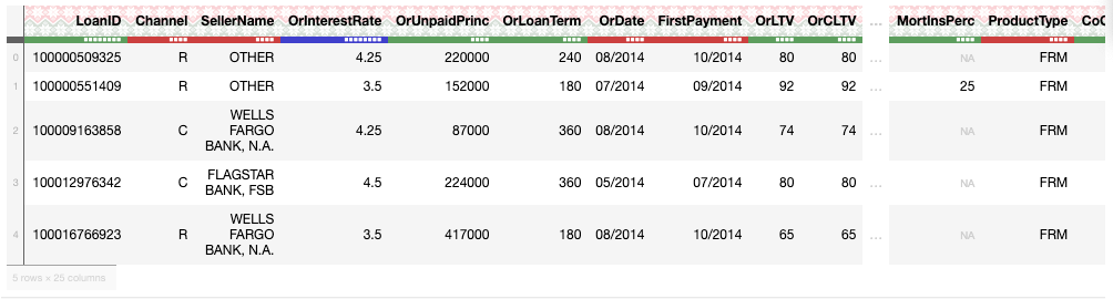

df_per.head(5))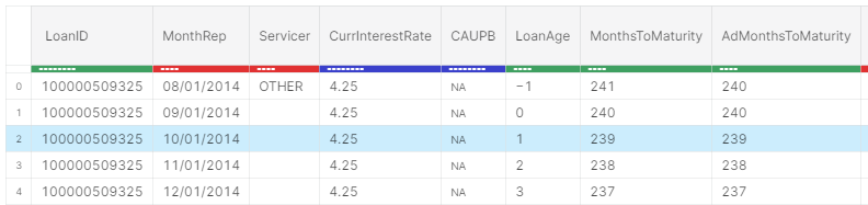

The color of the progress bar denotes the datatype where red denotes string, green denotes int and blue stands for float.

2. Data Preprocessing

In the Performance dataset , we are only interested in the LoanID  and ForeclosureDate  columns, as this will give us the borrower identification number and whether or not they ended up defaulting. 

• Selecting specific columns

So, let us select only the LoanID and the ForeclosureDate column and discard the rest

df_per = df_per[:,['LoanID','ForeclosureDate']]
df_per.head(5)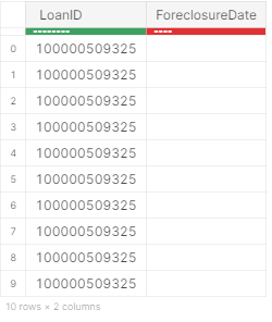

• Removing Duplicate entities

The Loan ID contains duplicated entities. Let’s also get rid of them.

dt.unique(df_per[:,"LoanID"]).head(5)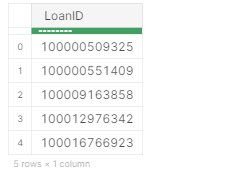

• Grouping

Let’s group the frame by unique Loan IDs. This will ensure that only unique Loan IDs exist in our dataset.

df_per = df_per[-1:,:, dt.by(dt.f.LoanID)]
df_per.head(5)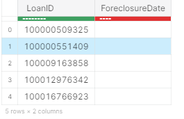

The f-expression supports arithmetic operations as well as various mathematical and aggregate functions.

• Joining the Acquisition and Performance Frames

Let’s now combine both the Acquisition and Performance frames by performing an inner join using theLoanID column. Let’s name the resulting dataframe, as df. This frame consists of theForeclosureDate column, and we shall be using it as our target variable . Let’s rename this column as Will_Default so as to avoid any confusion.

df_per.names = ['LoanID','Will_Default']
df_per.key = 'LoanID'
df= df_acq[:,:,dt.join(df_per)]

• Formatting the Target Column

The Will Default column consists of dates. For instance, if a borrower has paid the loan, then the date on which the loan was paid is mentioned. However, if the loan hasn’t been repaid, the field is left blank. Let’s replace the blank values with ‘0’ i.e the loan has never been paid and field with some values as ‘1’. This means the borrower has not defaulted i.e who has paid the loan on some date.

# Replacing the dates in the Will_Default column with '0' and null values with 1
df[:,'Will_Default'] = df[:, {'Will_Default': dt.f['Will_Default']==""}]
df.head(5)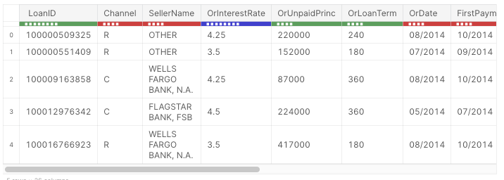

Finally, let’s look at the shape of the processed dataset.

df.shape
-------------------------------------------------------
(394356, 26)

The dataframe has 394356  rows and 26  columns and contains information regarding loan interest rate, payment dates, property state, and the last few digits of each property ZIP code, among several other things. From here the data is ready to be fed into a model for training purposes. One can also convert it into a Pandas dataframe, CSV file or into a binary. jay file as follows:

df.to_pandas()
df.to_csv("out.csv")
df.to_jay("data.jay")

Database-like ops benchmark

Today, a lot of database-like tools exist in the data science ecosystem. In an effort to compare their performance, a benchmark  has been created which runs regularly against the very latest versions of these packages and automatically updates. This is beneficial for both the developers of the packages as well as for the users. You can find out more about the project in Efficiency in data processing slides  and talk made by Matt Dowle on H2OWorld 2019 NYC conference .

Reading the benchmark

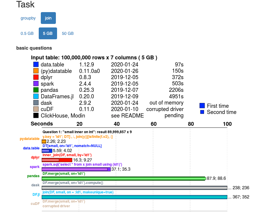
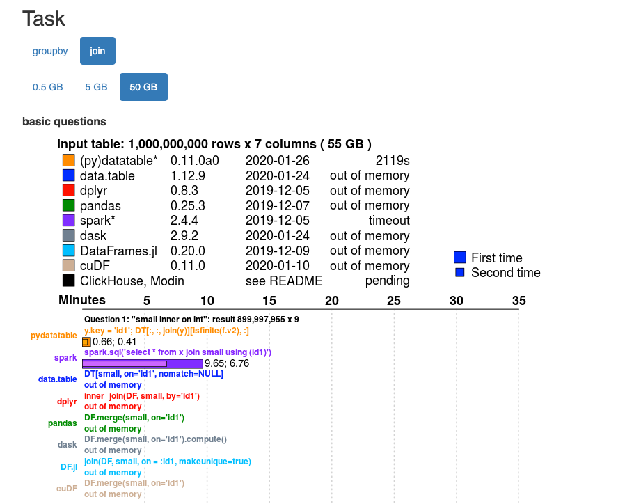
You can click the tab for the size of the data you have and for the type of operation being performed. You are then provided a side by side comparison of the various tools along with the time taken for the tasks. For instance below is the benchmark for the ‘join ’ function performed on a 5 GB and 50GB dataset, and as can be seen, datatable fares really well.

• 5GB dataset

• 50 GB dataset

Feel free to check out the page yourself for more tasks and other details:

Database-like ops benchmark

Conclusion

The datatable package really shines when working with big data. With its emphasis on big data support , datatable offers a lot of benefits and can really improve the time taken to performs data wrangling tasks on a dataset. Datatable is an open-source project and hence it is open to contributions and collaborations to improve it and make it even better.