Using Tabular Foundation Model in Driverless AI - TabPFN v2

1. Introduction

TabPFN (Prior-Fitted Network for Tabular data) is a foundation model for tabular prediction developed by Prior Labs. Unlike gradient-boosted trees that learn from scratch on every dataset, TabPFN is a transformer pre-trained on millions of synthetic tabular datasets. At inference time, it treats the entire training set as context and produces predictions in a single forward pass — no iterative optimization, no hyperparameter grid search.

TabPFN V2 supports up to 10,000 training rows, 500 features, and handles both classification (up to 10 native classes) and regression out of the box. 2 Motivation Traditional AutoML pipelines rely on ensembles of gradient-boosted trees (LightGBM, XG- Boost, CatBoost) that require per-dataset tuning. This works well at scale but has notable gaps:

2. Motivation

Traditional AutoML pipelines rely on ensembles of gradient-boosted trees (LightGBM, XG- Boost, CatBoost) that require per-dataset tuning. This works well at scale but has notable gaps:

• Small-data regime: With fewer than ˜10K rows, tree-based models are prone to over- fitting and their performance plateaus quickly. A pre-trained model that encodes prior knowledge about tabular structure can extract signal more reliably.
• Feature engineering pressure: TabPFN learns cross-feature interactions internally via attention, reducing the burden on hand-crafted or brute-force feature engineering.
• Ensemble diversity: Stacking benefits from base learners with fundamentally different inductive biases. A transformer-based model complements trees in ways that another tree variant cannot. 

The DAI TabPFN recipe targets exactly this niche: a high-accuracy base model for small-to- medium datasets that diversifies the ensemble.

3. Design in DAI

The TabPFN integration spans three recipe files, each registered as a DAI custom component:

The high level design of the recipes are inspired by or adapted from tabpfn-extensions, the official extension library maintained by Prior Labs.

3.1 TabPFNModel

TabPFNModel is the primary recipe. It registers as a CustomModel supporting binary, multiclass, and regression tasks.

Native mixed-type support: A key advantage of TabPFN as a DAI model is its ability to consume raw features directly — both categorical and numerical — without requiring elaborate preprocessing. Traditional tree-based pipelines in DAI rely on a complex chain of feature engi- neering, encoding, and imputation transformers before the model ever sees the data. TabPFN’s transformer architecture handles heterogeneous feature types natively through its learned at- tention mechanism, which significantly simplifies the end-to-end pipeline. This has practical benefits for production deployment: fewer pipeline stages mean fewer serialization artifacts, reduced latency in the scoring path, and a smaller surface area for bugs or version mismatches between training and serving environments.

Gating logic (can use):

This deliberately restricts the model to scenarios where it adds value — small datasets where accuracy matters and a GPU is present.

Finetuning: The recipe uses FinetunedTabPFNClassifier / FinetunedTabPFNRegressor from the TabPFN library. Instead of zero-shot inference, it fine-tunes the pre-trained V2 weights on the downstream dataset for a configurable number of epochs (finetune epochs) with a task-specific learning rate (finetune learning rate). This bridges the gap between generic priors and dataset-specific patterns.

Explanations: The recipe implements both global and local interpretability:

• Global : SAGE (Shapley Additive Global importancE) simulation using Permutation-Estimator with a MarginalImputer backed by a K-means coreset of the training data.
• Local : Shapley value computation (pred contribs) using the same permutation frame-work, computing feature contributions in logit space for consistency.

These are model-agnostic approaches — they do not exploit TabPFN’s internal attention weights. This is accurate but computationally expensive.

3.2 Hyperparameter Trade-offs

The recipe adapts hyperparameters to DAI’s accuracy dial:

Key intuition:

• Lower temperature sharpens predictions (more confident), useful at high accuracy where calibration is fine-tuned separately.

• More ensembles (n estimators) reduce variance at the cost of inference time.

• More finetuning epochs with lower LR at high accuracy allows careful adaptation without destroying pre-trained representations.

• balance probabilities and average before softmax improve calibration on imbalanced datasets — enabled when accuracy matters.

3.3 TabPFNEmbeddingTransformer

This transformer extracts learned embeddings from a fitted TabPFN model and reduces dimensionality via SVD. It produces numeric features that downstream models (e.g., LightGBM) can consume, effectively using TabPFN as a feature extractor.

Gated by: accuracy > 8, interpretability < 2, features <= 30, train rows < 20K. This is the most restrictive recipe — embedding extraction is expensive and only justified when pushing for maximum accuracy on small, low-dimensional datasets.

3.4 TabPFNOutlierScoreTransformer

An unsupervised transformer that estimates density via the chain rule over random feature permutations. Each row gets an outlier score: -log(max(p(x), eps)). The top-K features are selected via a surrogate Random Forest, and density-aware sampling ensures the model focuses on the distribution tails.

Gated by: features <= 15, train rows < 20K. The chain-rule density estimation scales combinatorially with feature count, so the conservative feature cap is essential.

4. Performance Comparison with LightGBM

We evaluated TabPFN against LightGBM on two binary classification datasets using LogLoss as the primary metric.

4.1 Insurance Fraud (˜12K rows, 6% positive rate)

TabPFN achieves better discrimination (AUC, AUCPR) while LightGBM has a marginal edge in calibration (LogLoss delta = 0.0005). The PR curve (Figure 1) shows TabPFN consistently above LightGBM across recall levels. Both models show tight generalization gaps (¡1% relative), indicating no overfitting.

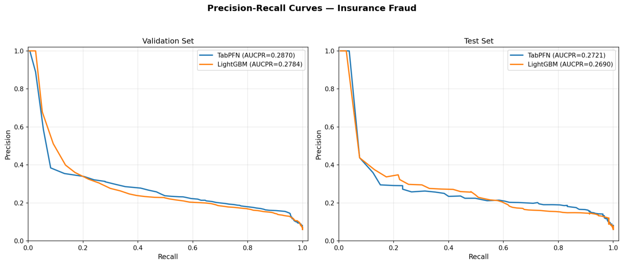
Figure 1: PR curve — Insurance Fraud dataset

The confusion matrices (Figure 2) reveal similar operating characteristics — both struggle with minority-class recall (˜43–49%) on this imbalanced dataset.

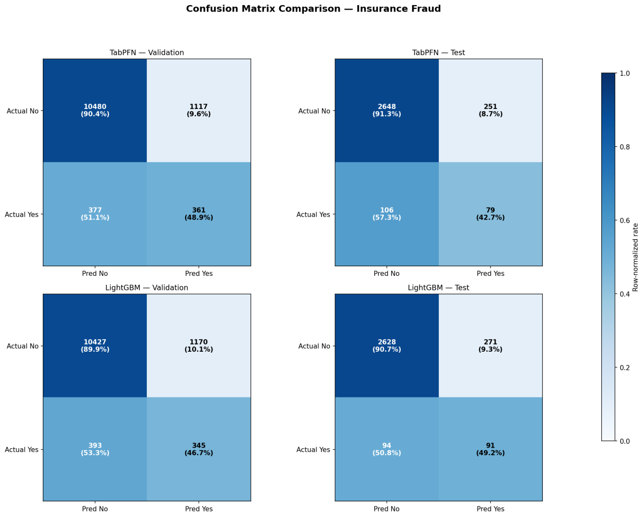
Figure 2: Confusion matrices — Insurance Fraud dataset

4.2 Kaggle Credit Card Fraud (˜20K rows, 0.17% positive rate)

Under extreme class imbalance, TabPFN generalizes significantly better. LightGBM overfits more on validation (46.7% relative generalization gap vs. TabPFN’s 11%). The confusion matrices (Figure 3) highlight the most striking difference: TabPFN catches 11/15 frauds (73% recall) vs. LightGBM’s 7/15 (47%) on the test set. The PR curve (Figure 4) confirms TabPFN’s superior AUCPR on test.

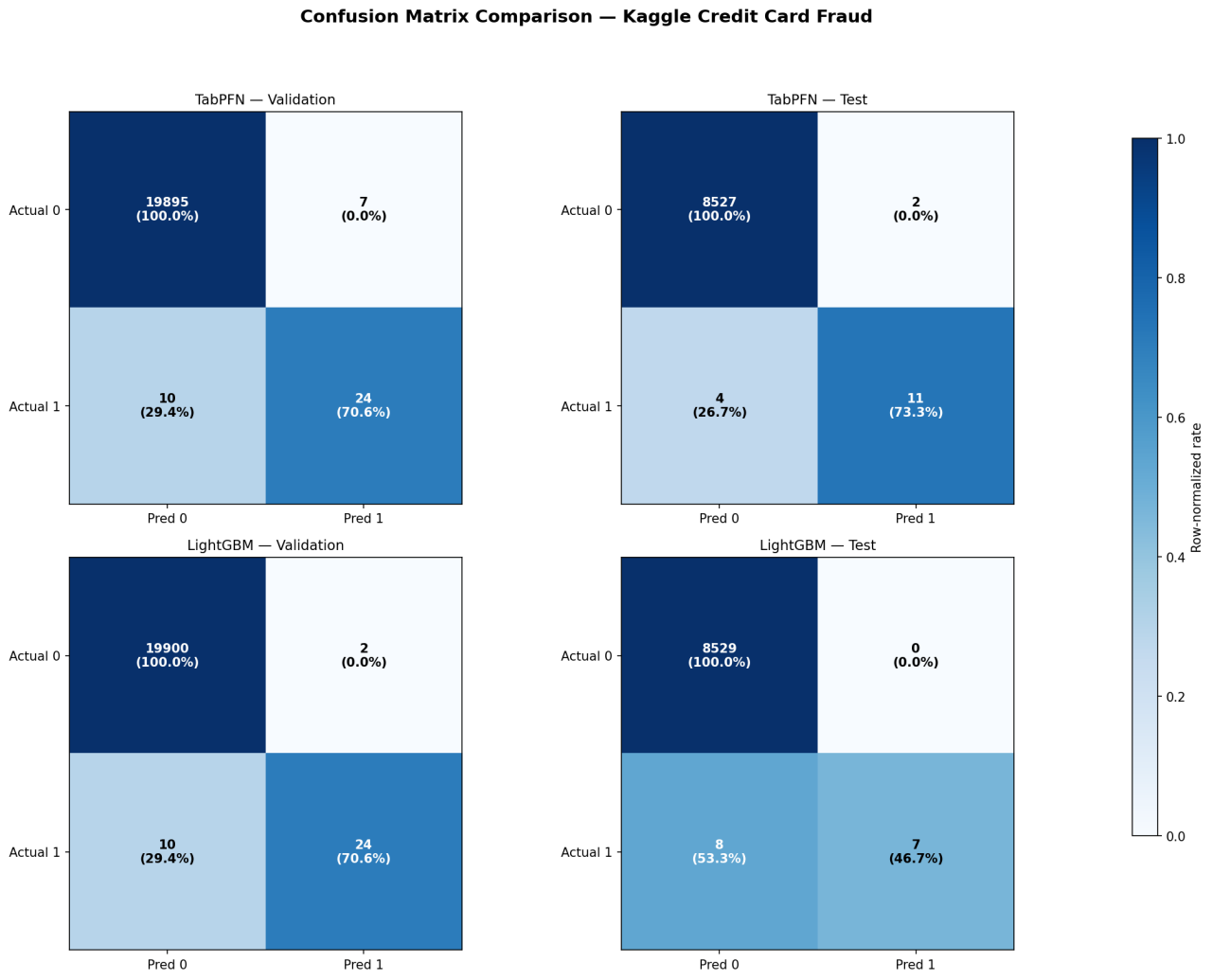
Figure 3: Confusion matrices — Kaggle Credit Card Fraud dataset

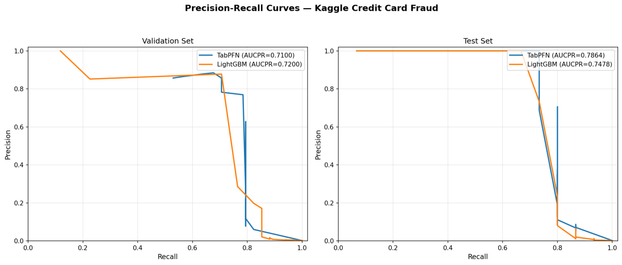
Figure 4: PR curve — Kaggle Credit Card Fraud dataset

5. Current Limitations

1. Training size cap: TabPFN is capped at 10,000 rows (TRAIN SIZE LIMITS). Datasets exceeding this are downsampled (stratified for classification), discarding potentially valuable data. The TRAIN SIZE OVERLOAD RATE = 2 allows up to 20K rows to enter the recipe, but the model still trains on a 10K subsample.
2. Interpretability cost: SAGE and Shapley computations are model-agnostic — they require hundreds of forward passes through the imputer. With MAX GLOBAL EXPLANATION PERMUTATIONS = 256 and MAX LOCAL EXPLANATION PERMUTATIONS = 32, explanation time can dwarf training time. For ¿100 features, the recipe falls back to uniform importance. This is the primary bottleneck for production deployment where explanations are mandatory.
3. GPU requirement: All three recipes set must use gpu = True. There is no CPU fallback, limiting deployment to GPU-equipped environments.
4. No sample weight support: supports sample weight = False prevents integration with DAI’s built-in sample weighting, which can be important for cost-sensitive or imbalanced learning.
5. No MOJO export: The embedding and outlier transformers set mojo = False, preventing low-latency scoring pipeline deployment for recipes that include these transformers.

6. Future Work

1. TabICL V2 for large datasets: TabICL is a complementary in-context learning model designed specifically for larger tabular datasets (100K+ rows). Integrating TabICL V2 as an additional recipe would remove the 10K row ceiling while preserving the in-context learning paradigm.
2. Higher inference speed: The current SAGE/Shapley explanation path is the primary bottleneck. Future work could explore attention-based attribution (extracting importances directly from TabPFN’s internal attention maps) to replace the model-agnostic permutation approach, potentially reducing explanation time by an order of magnitude.
3. Improved embeddings: The current TabPFNEmbeddingTransformer extracts representations post-hoc via SVD. A tighter integration — such as intermediate-layer feature extraction or contrastive fine-tuning of embeddings — could produce richer features for downstream models.
4. Broader recipe interoperability: Enabling sample weight support and MOJO export would allow TabPFN recipes to participate more fully in DAI’s optimization and deployment pipelines.
5. Target imputation for time series: TabPFN’s pre-trained conditional distribution can serve as a principled imputation model for missing target values. This is particularly relevant for time series forecasting in DAI, where gaps between the end of training history and the forecast horizon cause lag features to become entirely NaN — degrading Test Time Augmentation (TTA) performance. A TabPFN-backed imputer could fill these gaps causally (conditioning only on past observations), producing more informative lag features and improving forecast accuracy on long-horizon prediction problems.

References

• TabPFNModel

• TabPFNOutlierScoreTransformer

• TabPFNEmbeddingTransformer

• Kaggle Fraud dataset

• Insurance Fraud dataset