H2O is a scalable and open-source math and machine learning platform for big data. It can handle much bigger datasets and run a lot faster than R/SAS even on a single machine. How does the modeling experience with H2O differ from the experience using traditional tools such as R/SAS? This blog answers exactly this question. In particular, I will show you how 10 minutes of practice in H2O could put you on a solid path (fast track) to win the KDDCup98 data mining competition.

The goal of the KDDCup98 competition is to maximize donation from a pool of potential donors for a non-profit organization. It costs the organization $0.68 to process and send a campaign letter to each prospect. Due to this cost, the organization wants to predict how much each potential donor is likely to contribute. If the forecasted donation is less than $0.68 for a donor, he/she will be skipped from the campaign. In marketing, this type of problem is called lead scoring and often needs to be addressed by almost every marketing organization today. In recent 3 years, there are at least a dozen startups that are funded to work on this type of problem. So although the KDDCup98 competition is more than 15 years old, the problem it addresses is still very useful in practice.
Let’s get started.

Download & Start H2O

H2O can be downloaded from its website www.h2o.ai/download/. For this example, we use the Maxwell release. Assume the downloaded file is at ~/Downloads (as on Mac computers), you can unzip and start H2O by typing the following commands from your terminal:

cd ~/Downloads
unzip h2o-2.8.2.8.zip
cd h2o-2.8.2.8
java -jar h2o.jar

Now point your browser to http://localhost:54321, you will see the H2O web interface.
 

Download Data

The training and test datasets for KDDCup98 can be downloaded from http://data.h2o.ai/usecases/cup98LRN_z.csv (as training dataset) and http://data.h2o.ai/usecases/cup98VAL_z.csv (as test dataset). The training dataset has about 95K rows and 481 columns. Three of the columns are special:

• CONTROLN: control number. The id column.
• TARGET_B: binary. Whether the donor responded to the campaign.
• TARGET_D: numeric. The amount of money that a donor contributes.

The original test data has about 96K rows and 479 columns (missing the TARGET_B and TARGET_D). A separate file with the target columns was provided after the competition. We have merged the two files so in the download data, the test dataset also has 481 columns.

Modeling with H2O

Modeling with H2O using the web interface is fairly easy. It usually involves only a few steps:
** Step 1 ** Upload files. In the web interface, select Data→Upload, then select the training data file.
 
After selecting the file, click on “Upload” to upload the file.
 
The next screen shows the preliminary parsing result. H2O automatically recognized the file type (comma-separated), header, and shows a preview of the data. Pay some attention to the “destination key” field, which has a default value of cup98LRN_z.hex. This is the key we will use to identify this dataset.
 
Click “Submit”, the file will be parsed. You will see the Inspect2 screen. The bottom portion of the screen shows summaries for each column and sample data. Notice the “As Factor” buttons for column ODATEDW, TCODE, etc. “As Factor” means such columns are treated as numerical columns. We want to change the first 7 such columns to categorical. Simply click on the “As factor” buttons below these columns:

• ODATEDW
• TCODE
• ZIP
• DOB
• NOEXCH
• CLUSTER
• AGE

setwd("$PATH_TO_DATA_FILES")
kdd98 <- read.csv("cup98VAL_z.csv") # read data
kdd_pred = read.csv("drf_predict.csv") # read prediction value
kdd_pred_val <- apply(kdd_pred,1,function(row) if (row[1] > 0.68) 1 else 0 )
kdd98_withpred <- cbind(kdd98, kdd_pred_val)
kdd98_withpred$yield <- apply(kdd98_withpred,1,function(row) (as.numeric(row['TARGET_D']) - 0.68) * as.numeric(row[483]))
sum(kdd98_withpred$yield) # profit
sum(kdd_pred_val) # mails sent

The last two lines of code reports the profit from the campaign ($14,446.26) and the # of mails sent (52,117). Your results may be slightly different due to randomness.
The profit number $14,446.26 will rank #3 in the competition, and is only about $266 less than the best result.
 

Modeling with R

What’s significant about the modeling with H2O is that we did not do anything special to reach #3 in the competition: no sampling, no feature selection , and no special treatment for missing values. We simply used out-of-the-box H2O, then fed it with all the training data. Let’s now look at how R fares in this case.
One of the most popular random forest package in R is randomForest. If we simply run random forest on the KDDCup98 training dataset,

kdd98 <- read.csv("cup98LRN_z.csv") # read data
features <- setdiff(colnames(kdd98), c("CONTROLN", "TARGET_B"))
kdd98 <- kdd98[, features] # remove id columns and TARGET_B
library(randomForest)
rf <- randomForest(TARGET_D ~ ., data=kdd98)

We receive an error “missing values in object”. randomForest cannot handle missing values. Even if we impute the missing values, we will encounter the next roadblock: the package does not support categorical variables with more than 32 levels.
Another R package “party” does not have these limitations. However, when we run it with

library(party)
cf <- cforest(TARGET_D ~ ., data= kdd98, control = cforest_unbiased(mtry=2, ntree=50))

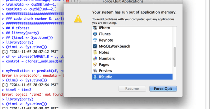
My R instance is using 8GB+ memory and eventually runs out of application memory:
 
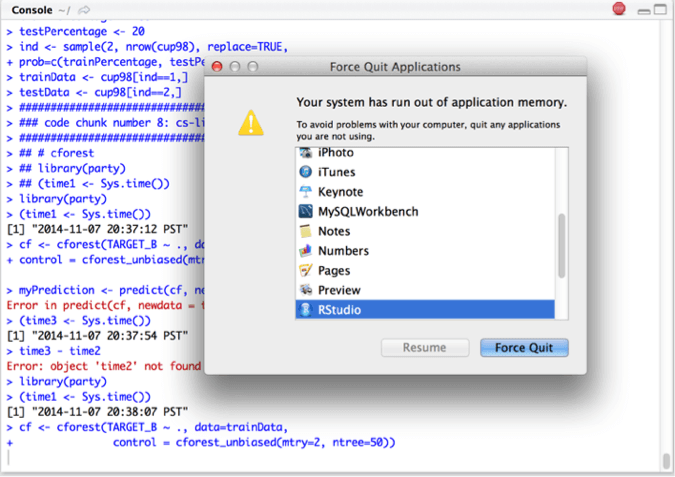
I then engaged in a round of feature selection, using only 64 (instead of 478) columns in modeling. Unfortunately, cforest failed to return after 6 hours.
This shows that even with moderate amount of data, R may fail to build a model. H2O can handle larger amount of data really fast: the model runs less than 2 minutes with all the data.

What’s Better: Combining R and H2O

While R may not be suitable for building large scale machine learning models, it is superb for data pre-processing and post-processing. In our H2O modeling example, the Evaluation step was done in R. R is also great for automating the modeling flow. If you want to rerun your model, using the web interface may be cumbersome as you have to re-enter the selections you made before.
What is great for H2O is that it supports an R interface. H2O offers an R package that can be installed from CRAN. Once installed, you can let R do the data munging work and delegate to H2O for heavy-duty model building. The model building and scoring process we developed with H2O web interface can be achieved equally for our KDDCup98 demo using the H2O package in R.
As a real-life example combining R and H2O, Cisco is now using H2O to regularly run 60K+ ensemble models on datasets with more than 160M rows and 1000+ attributes. R is used as a gateway to manage all the models for data scientists. You may find the details in another blog at http://www.h2o.ai/blog/2014/11/predictive-modeling-at-scale/