This post is reposted from Rstudio’s announcement on sparklyr – Rstudio’s extension for Spark

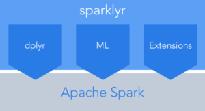
- Connect to Spark from R. The sparklyr package provides a complete dplyr backend.
- Filter and aggregate Spark datasets then bring them into R for analysis and visualization.
- Use Spark’s distributed machine learning library from R.
- Create extensions that call the full Spark API and provide interfaces to Spark packages.
Installation
You can install the sparklyr package from CRAN as follows:
install.packages("sparklyr")
You should also install a local version of Spark for development purposes:
library(sparklyr)
spark_install(version = "1.6.2")
To upgrade to the latest version of sparklyr, run the following command and restart your r session:
devtools::install_github("rstudio/sparklyr")
If you use the RStudio IDE, you should also download the latest preview release of the IDE which includes several enhancements for interacting with Spark (see the RStudio IDE section below for more details).
Connecting to Spark
You can connect to both local instances of Spark as well as remote Spark clusters. Here we’ll connect to a local instance of Spark via the spark_connect function:
library(sparklyr)
sc <- spark_connect(master = "local")
The returned Spark connection (sc) provides a remote dplyr data source to the Spark cluster.
For more information on connecting to remote Spark clusters see the Deployment section of the sparklyr website.
Using dplyr
We can new use all of the available dplyr verbs against the tables within the cluster.
We’ll start by copying some datasets from R into the Spark cluster (note that you may need to install the nycflights13 and Lahman packages in order to execute this code):
install.packages(c("nycflights13", "Lahman"))
library(dplyr)
iris_tbl <- copy_to(sc, iris)
flights_tbl <- copy_to(sc, nycflights13::flights, "flights")
batting_tbl <- copy_to(sc, Lahman::Batting, "batting")
src_tbls(sc)
## [1] "batting" "flights" "iris"
To start with here’s a simple filtering example:
# filter by departure delay and print the first few records
flights_tbl %>% filter(dep_delay == 2)
## Source: query [?? x 19]
## Database: spark connection master=local[8] app=sparklyr local=TRUE
##
## year month day dep_time sched_dep_time dep_delay arr_time
## <int> <int> <int> <int> <int> <dbl> <int>
## 1 2013 1 1 517 515 2 830
## 2 2013 1 1 542 540 2 923
## 3 2013 1 1 702 700 2 1058
## 4 2013 1 1 715 713 2 911
## 5 2013 1 1 752 750 2 1025
## 6 2013 1 1 917 915 2 1206
## 7 2013 1 1 932 930 2 1219
## 8 2013 1 1 1028 1026 2 1350
## 9 2013 1 1 1042 1040 2 1325
## 10 2013 1 1 1231 1229 2 1523
## # ... with more rows, and 12 more variables: sched_arr_time <int>,
## # arr_delay <dbl>, carrier <chr>, flight <int>, tailnum <chr>,
## # origin <chr>, dest <chr>, air_time <dbl>, distance <dbl>, hour <dbl>,
## # minute <dbl>, time_hour <dbl>
Introduction to dplyr provides additional dplyr examples you can try. For example, consider the last example from the tutorial which plots data on flight delays:
delay <- flights_tbl %>%
 group_by(tailnum) %>%
 summarise(count = n(), dist = mean(distance), delay = mean(arr_delay)) %>%
 filter(count > 20, dist < 2000, !is.na(delay)) %>%
 collect
# plot delays
library(ggplot2)
ggplot(delay, aes(dist, delay)) +
 geom_point(aes(size = count), alpha = 1/2) +
 geom_smooth() +
 scale_size_area(max_size = 2)
Window Functions
dplyr window functions are also supported, for example:
batting_tbl %>%
 select(playerID, yearID, teamID, G, AB:H) %>%
 arrange(playerID, yearID, teamID) %>%
 group_by(playerID) %>%
 filter(min_rank(desc(H)) <= 2 & H > 0)
## Source: query [?? x 7]
## Database: spark connection master=local[8] app=sparklyr local=TRUE
## Groups: playerID
##
## playerID yearID teamID G AB R H
## <chr> <int> <chr> <int> <int> <int> <int>
## 1 abbotpa01 2000 SEA 35 5 1 2
## 2 abbotpa01 2004 PHI 10 11 1 2
## 3 abnersh01 1992 CHA 97 208 21 58
## 4 abnersh01 1990 SDN 91 184 17 45
## 5 abreujo02 2014 CHA 145 556 80 176
## 6 acevejo01 2001 CIN 18 34 1 4
## 7 acevejo01 2004 CIN 39 43 0 2
## 8 adamsbe01 1919 PHI 78 232 14 54
## 9 adamsbe01 1918 PHI 84 227 10 40
## 10 adamsbu01 1945 SLN 140 578 98 169
## # ... with more rows
For additional documentation on using dplyr with Spark see the dplyr section of the sparklyr website.
Using SQL
It’s also possible to execute SQL queries directly against tables within a Spark cluster. The spark_connection object implements a DBI interface for Spark, so you can use dbGetQuery to execute SQL and return the result as an R data frame:
library(DBI)
iris_preview <- dbGetQuery(sc, "SELECT * FROM iris LIMIT 10")
iris_preview
## Sepal_Length Sepal_Width Petal_Length Petal_Width Species
## 1 5.1 3.5 1.4 0.2 setosa
## 2 4.9 3.0 1.4 0.2 setosa
## 3 4.7 3.2 1.3 0.2 setosa
## 4 4.6 3.1 1.5 0.2 setosa
## 5 5.0 3.6 1.4 0.2 setosa
## 6 5.4 3.9 1.7 0.4 setosa
## 7 4.6 3.4 1.4 0.3 setosa
## 8 5.0 3.4 1.5 0.2 setosa
## 9 4.4 2.9 1.4 0.2 setosa
## 10 4.9 3.1 1.5 0.1 setosa
Machine Learning
You can orchestrate machine learning algorithms in a Spark cluster via the machine learning functions within sparklyr . These functions connect to a set of high-level APIs built on top of DataFrames that help you create and tune machine learning workflows.
Here’s an example where we use ml_linear_regression to fit a linear regression model. We’ll use the built-in mtcars dataset, and see if we can predict a car’s fuel consumption (mpg) based on its weight (wt), and the number of cylinders the engine contains (cyl). We’ll assume in each case that the relationship between mpg and each of our features is linear.
# copy mtcars into spark
mtcars_tbl <- copy_to(sc, mtcars)
# transform our data set, and then partition into 'training', 'test'
partitions <- mtcars_tbl %>%
 filter(hp >= 100) %>%
 mutate(cyl8 = cyl == 8) %>%
 sdf_partition(training = 0.5, test = 0.5, seed = 1099)
# fit a linear model to the training dataset
fit <- partitions$training %>%
 ml_linear_regression(response = "mpg", features = c("wt", "cyl"))
fit
## Call: ml_linear_regression(., response = "mpg", features = c("wt", "cyl"))
##
## Coefficients:
## (Intercept) wt cyl
## 37.066699 -2.309504 -1.639546
For linear regression models produced by Spark, we can use summary() to learn a bit more about the quality of our fit, and the statistical significance of each of our predictors.
summary(fit)
## Call: ml_linear_regression(., response = "mpg", features = c("wt", "cyl"))
##
## Deviance Residuals::
## Min 1Q Median 3Q Max
## -2.6881 -1.0507 -0.4420 0.4757 3.3858
##
## Coefficients:
## Estimate Std. Error t value Pr(>|t|)
## (Intercept) 37.06670 2.76494 13.4059 2.981e-07 ***
## wt -2.30950 0.84748 -2.7252 0.02341 *
## cyl -1.63955 0.58635 -2.7962 0.02084 *
## ---
## Signif. codes: 0 '***' 0.001 '**' 0.01 '*' 0.05 '.' 0.1 ' ' 1
##
## R-Squared: 0.8665
## Root Mean Squared Error: 1.799
Spark machine learning supports a wide array of algorithms and feature transformations and as illustrated above it’s easy to chain these functions together with dplyr pipelines. To learn more see the machine learning section.
Reading and Writing Data
You can read and write data in CSV, JSON, and Parquet formats. Data can be stored in HDFS, S3, or on the lcoal filesystem of cluster nodes.
temp_csv <- tempfile(fileext = ".csv")
temp_parquet <- tempfile(fileext = ".parquet")
temp_json <- tempfile(fileext = ".json")
spark_write_csv(iris_tbl, temp_csv)
iris_csv_tbl <- spark_read_csv(sc, "iris_csv", temp_csv)
spark_write_parquet(iris_tbl, temp_parquet)
iris_parquet_tbl <- spark_read_parquet(sc, "iris_parquet", temp_parquet)
spark_write_csv(iris_tbl, temp_json)
iris_json_tbl <- spark_read_csv(sc, "iris_json", temp_json)
src_tbls(sc)
## [1] "batting" "flights" "iris" "iris_csv"
## [5] "iris_json" "iris_parquet" "mtcars"
Extensions
The facilities used internally by sparklyr for its dplyr and machine learning interfaces are available to extension packages. Since Spark is a general purpose cluster computing system there are many potential applications for extensions (e.g. interfaces to custom machine learning pipelines, interfaces to 3rd party Spark packages, etc.).
Here’s a simple example that wraps a Spark text file line counting function with an R function:
# write a CSV
tempfile <- tempfile(fileext = ".csv")
write.csv(nycflights13::flights, tempfile, row.names = FALSE, na = "")
# define an R interface to Spark line counting
count_lines <- function(sc, path) {
 spark_context(sc) %>%
 invoke("textFile", path, 1L) %>%
 invoke("count")
}
# call spark to count the lines of the CSV
count_lines(sc, tempfile)
## [1] 336777
To learn more about creating extensions see the Extensions section of the sparklyr website.
dplyr Utilities
You can cache a table into memory with:
tbl_cache(sc, "batting")
and unload from memory using:
tbl_uncache(sc, "batting")
Connection Utilities
You can view the Spark web console using the spark_web function:
spark_web(sc)
You can show the log using the spark_log function:
spark_log(sc, n = 10)
## 16/09/24 07:50:59 INFO ContextCleaner: Cleaned accumulator 224
## 16/09/24 07:50:59 INFO ContextCleaner: Cleaned accumulator 223
## 16/09/24 07:50:59 INFO ContextCleaner: Cleaned accumulator 222
## 16/09/24 07:50:59 INFO BlockManagerInfo: Removed broadcast_64_piece0 on localhost:56324 in memory (size: 20.6 KB, free: 483.0 MB)
## 16/09/24 07:50:59 INFO ContextCleaner: Cleaned accumulator 220
## 16/09/24 07:50:59 INFO Executor: Finished task 0.0 in stage 67.0 (TID 117). 2082 bytes result sent to driver
## 16/09/24 07:50:59 INFO TaskSetManager: Finished task 0.0 in stage 67.0 (TID 117) in 122 ms on localhost (1/1)
## 16/09/24 07:50:59 INFO DAGScheduler: ResultStage 67 (count at NativeMethodAccessorImpl.java:-2) finished in 0.122 s
## 16/09/24 07:50:59 INFO TaskSchedulerImpl: Removed TaskSet 67.0, whose tasks have all completed, from pool
## 16/09/24 07:50:59 INFO DAGScheduler: Job 47 finished: count at NativeMethodAccessorImpl.java:-2, took 0.125238 s
Finally, we disconnect from Spark:
spark_disconnect(sc)
RStudio IDE
The latest RStudio Preview Release of the RStudio IDE includes integrated support for Spark and the sparklyr package, including tools for:
- Creating and managing Spark connections
- Browsing the tables and columns of Spark DataFrames
- Previewing the first 1,000 rows of Spark DataFrames
Once you’ve installed the sparklyr package, you should find a new Spark pane within the IDE. This pane includes a New Connection dialog which can be used to make connections to local or remote Spark instances:

Once you’ve connected to Spark you’ll be able to browse the tables contained within the Spark cluster:

The Spark DataFrame preview uses the standard RStudio data viewer:

The RStudio IDE features for sparklyr are available now as part of the RStudio Preview Release .


