Replay: Modeling MNIST With RF Hands-on Demo

Last week Spencer put together a great hands on for modeling data using H2O (http://www.meetup.com/H2Omeetup/).  This post is a write-up of the workflow for generating an RF model on MNIST data for those of you who want to walk through the demo again, or maybe missed the live action version.  I’m running through one of our local servers, with an allocation to H2O of 20 gigs.
RF on MNIST data: Spencer used a data set of pre-GPUed MNIST data similar to that provided by Kaggle in a currently running competition.  If you’re interested in some of the different approaches to the MNIST data (including Neural Nets and K Nearest Neighbors) I highly recommend taking a look at http://yann.lecun.com/exdb/mnist/.
Problem: The training data are 60,000 observations of 786 variables, testing data are 10,000 observations. Each independent variable corresponds to one square pixel of  an image. The value given for any variable indicates the level of saturation of the pixel.  Results are given and discussed below. Here is the step by step process for generating these results.

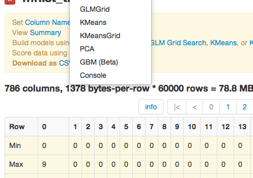
1. Starting at the drop down menu Data inhale and parse data (both the testing and training sets).
2. From the Model drop down menu choose **Random Forest**
   
3. Set Ntree = 50, and Features = 200. Leave all other options in default.  Note that H2O automatically ignores all constant columns, so you need not sort through the data summary by hand  to find those variables.
4. Step 3 generates a model, the confusion matrix shown below is the output of this model.
5. The model key is at the top of the RF results page; highlight and copy it. From the drop down menu Score, select RF.
6. In the specification page for scoring your RF model enter the .hex  key for your testing data, paste the model key, specify the dependent variable column, and submit.

At this point you have built a model and verified that it works. In practice, the motivation is generally to actually predict an outcome of interest – which you can now do with this same model by returning to the drop down menu Score and selecting Predict. Feeding  Predict data with the same predictors as contained in your training set produces a column of predictions matching each observation.
Results:  In an RF model of 50 trees,  features set to 200, and all other options left in default, H2O produces this confusion matrix.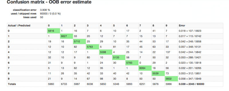
Testing the generated RF model on the test set  produces a classification error of 3.28%.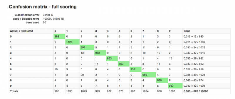
So- there you have it. A walkthrough of Spencer’s meetup presentation that you can follow step by step.