H2O World 2015, Day 1 Contribute to H2O open source machine learning software 

 

 

Talking Points:

• Decisions Trees: Concept
• Robust to Feature Distributions
• Decision Trees: Ensembles
• Random Forest
• Gradient Boosted Machines (GBM)
• Trees in H2O
• Demonstration with Python Model
• Demonstration with GBM Model
• Summary Found in Flow
• Q/A with Mark

 

Speakers:

Mark Landry, Data Scientist & Product Mgr, H2O

• LinkedIn

Read the Full Transcript

 

 

 

Moderator:

The next talk we have is Mark Landry. He's one of our data scientists at H2O Professional Kaggler and all around smart guy. This is going to be Gradient Boosting Methods as well as Random Forest. These are basically all tree methods, and so there's a data type that we're using a number of times in a number of these demos called cover type, looking at tree coverage. Just so happens that the tree methods for this particular data set also happen to work well and be quite strong on that. You'll see some of the better scores on that same data type. This talk is done I think we have a version of this in IPy notebook as well as Python as well as R, and so you should be able to follow along with whatever your preferred tool is.

Mark Landry:

Okay, thanks, Brandon. Okay, as he said, we're going to look at GBM and Random Forest in H2O. We'll look at it conceptually, and then we'll look at how our implementations work. We'll start with an algorithm background, they're both decision tree methods, so these are based on decision trees. We'll take a look at what those are and then the two implementations that sit on top of them, which are random forest and Gradient Boosted Machines. Then we'll look at the H2O implementation through code. We'll go through some of the parameters there. We'll go through a few models and show the difference in why those parameters might or might not be good choices. Going conceptually, decision trees are solving a model very differently than our classic vanilla linear model. They're going to separate the data according to a series of questions, is how I think of it.

Decisions Trees: Concept

As the age greater than 9.5 or not, it doesn't matter. 10 and 11, and 12 are all equivalent. They're all greater. It's going to subdivide the data set, move things left and right and build this tree model out that goes very deep to try to fit all the data. The big thing about decision trees is the questions are found automatically to optimize the separation of the data points by whatever you're trying to find. We have classification and regression trees. This is a simple example over here of looking through who survived the Titanic and the first thing it looked like the most of trying to divide the data, say you're going to get the most power up front in this example of the gender being male. Yes goes one way, and then of the males will subdivide on the age whether they're greater than 9.5 or not.

The females will go a different way, so you can think of that being every time it's going to subdivide the data, but you're going to ask a different question. You may wind up asking the same question and with the same cut point of many of these data points, but the decision tree continues to be independent. Practically, they have a lot of strengths. The biggest one would be that it is nonlinear, so it can actually be a really big strength. A lot of data is nonlinear, especially, with its correlation as far as the target you're trying to solve in particular. A good example of using the age example, maybe young people and older people have a similar rate of surviving, and in the middle range, they don't. That's a nonlinear relationship you can't fit that very well with a single coefficient. But decision trees will fit that very well.

They'll figure out what the best way to divide the young people, the middle people and the old people. They can handle that nonlinear relationship. They're very robust, so there's three listed here. We have correlated features. Two things that mean almost the same thing. You can think of maybe a zip code and a city if you're looking across the whole world or at least country maybe pretty tightly correlated. Af lot of people will look at a linear model as trying to break apart that correlation. Maybe they're going to throw it through PCA or maybe they're going to do a little more hands on to remove that because linear models are typically not great when you have that collinear features. But trees handle that very gracefully, it doesn't really matter to them. They'll keep looking through all of the available fields, all the available values and choose the best one.

Robust to Feature Distributions

Robust to feature distributions are kind of the same thing. They're working on that continuum. You can think 9.5, like I said, 10, 11, 12, 13, 20, they're all greater than 9.5 so the distribution doesn't really matter. Now in practice with the implementations, it can matter a slight bit, but for the most part you can think hands off of trying to apply a standard scaler to get my data into be a normal distribution for all of the predictors, which is a very common practice for most algorithms in robust to missing values. If you don't have values, the trees are okay. Again, different implementations handle at different ways, but they're all pretty good at handling this case. You do not have to impute, you can try that, you see if that works. You can do some other strategies, but they're very robust to working with missing values. For a lot of people, this makes it really practical for just getting started without handling some of these features. Simple to comprehend a little bit you can see how it works and in a human sense. Fast to train, faster to score at least an individual one. These are properties that people like about them. However, on the right side we have weaknesses, and number one is a big one. They're not that accurate, they're not bad, but they're not really competitive with a regularized linear model with deep learning.

Even some SVMs, even a naive baye sometimes will usually beat a single decision tree. They also can't project, it's a small one, doesn't get cited a lot. But if you think in time series if you have something that is inflation adjusted pricing and you want to predict the next one, a decision tree simply cannot predict outside the bounds that it was told of what a target was. Projecting means that I've passed you all these data points and you've understood this relationship, so that you can actually react to any set of data and do the right thing. Trees will keep predicting the max or min value at best. Usually, not much of an issue in data but in some cases that's something you want to be cognizant of what they're doing. On that same linear issue, we said it's nonlinear is a good thing. However, if you have a linear relationship as a predominant factor in your data set the decision tree will fit that, but it's going to do so very efficiently by trying to find all these cuts. Is it greater than nine? Maybe, the next one is, is it greater than 15? Is it less than 15? It's going to keep moving around that continuum just inefficient how it treats that.

Decision Trees: Ensembles

We can get away from the number one weakness, which is accuracy by putting them in as collections of them, which is ensembles and that's where we come. Random forest on the left GBM on the right, these are both ensemble tree algorithms. It's a way of combining multiple trees to solve the same problem. We have two different strategies here on the left we have random forest, which is bagging, that's bootstrap aggregation. What that really means is we're going to fit many different trees entirely, but on different samples of the data. We're going to shuffle the data around a little bit, grow a full tree and get answers to that, and then shuffle the data around a different way and grow a new tree. Then combine the results of each of the trees. And that definitely helps the predictive accuracy. The trees themselves are independent and that's just the GBM uses boosting.

Boosting is a little different, they're not independent anymore. These are dependent trees. And what it does is it will first guess the average of your value, and then figure out how good the average was and look at the difference between the average. The difference is really meaning a cost function, but can be thought of as a difference, and it's going to fit a tree to the differences. And then, it'll score that and it'll fit another tree on the differences of everything else. Each new tree is fixing up the differences of the entire system before it. It gets pretty complex and it's continually moving around where it was wrong the most. It tries to attack those, find patterns, create a tree that fits that and move on and then cycle through again. Two different strategies of how you can use trees in different ways. And these would by far be the most common implementations of ensemble tree methods.

Random Forest

Random forest specifically, at a little deeper it's going to combine our emotional decision trees, that I have stated, again. It's going to randomly sample the rows and the columns. There's standard, for that we implement the standards 63% of the rows is typical cut you'll take. The columns we have that set to where the for regression problem, it's going to be the square root of the number of columns you have. That's how many columns are going to be used to fit each model. That's a pretty small number. And classification, we're going to take 30%. You're going to see nowhere near the full amount of data then, but you're just going to keep fitting more and more trees. And the more trees you add the better these the system gets. Classically, you hear this a lot, it will reduce variance but with just a minimal increase in bias and that's where it gets a lot of its power.

In practical usage of random forest has a lot of strength. It's very easy to use, perhaps the easiest algorithm because it inherits all of those nice properties of the decision trees. And then, we add on accuracy by adding a few more things, and yet it's still just as easy to use as decision tree. There's very few hyper parameters to tune with a random forest. And for those parameters, there's well established defaults. Effectively, the two I told you maybe one more with depth. But we have standards that pretty much everybody uses and they're not too sensitive to those settings either. In the entire system of doing this bagging of the decision trees still winds up just as robust as decision trees themselves. Inherits all of that and very competitive. The accuracy is much better than an individual decision tree.

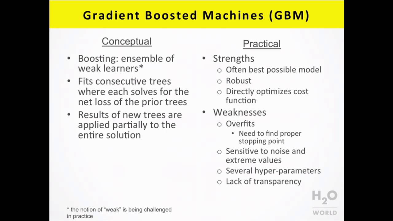
It's not uncommon to see a decision tree land at something like a low 70%, and a random forest wind up in the upper eighties or lower nineties as far as maybe a simple accuracy or something like that. Very common, so they're very powerful. Weaknesses are that they're slower to score because now we're actually fitting many, many trees and lack of transparency. And truthfully, in a decision tree you start to lose transparency when you get deep in there as well. But it's amplified by the fact that we're going to fit 30, 50, a hundred of these trees, so to wonder what this entire system of trees is doing is pretty hard. GBM a little deeper on that, so boosting is thought of as an ensemble of weak learners. I'm asterisk there because weak isn't really a thing. What that really is meaning is in this case, and actually I should say this first too, boosting can be applied to anything.

Gradient Boosted Machines (GBM)

They're just almost always applied to decision trees, and that's our implementation here. That's the most common implementation anywhere. In a case of a decision tree, what we'll do is just ask it less questions. We'll fit a very course model maybe four or five questions per data point, and score it and move on to the next one. Each one isn't very good, it's just not changing the average very much. But after you add more and more and more of these and it keeps focusing on the error you can actually get a really strong model after the end of it. And now, what we're seeing is actually people are getting very big decision trees, the depth I'm used to using four to eight maybe on these trees and now I'm seeing that 15 and 20 actually works really well. It almost looks like a random forest.

The last one, the results of the new trees are applied partially the entire solution. Part of what makes this algorithm work is that it's not just going to fix up all the errors that wouldn't work otherwise the first one would've been able to do it or a regular decision tree would work pretty well. It's going to work in partially, so the default way you apply the new tree is you take 10% of those predictions and apply it to the entire system. You're going to keep moving forward with a prediction where you add the results of each of these trees which can be negative. You can add subtract but you're doing it only in small forms. Even though this thing fits a number, you're going to take just a portion of that number and apply it and then fit a new tree and you're going to keep doing this.

It's strong in a practical sense that it's often the best possible model. It'll be deep learning in a lot of settings it'll be random forest in most settings though, the two are usually very close and it'll be a linear model in almost all settings. It's very, very, very high performing model or algorithm, I guess you say. Still robust, so it's still very easy to use, maybe a little less so than random forest takes a little tuning we'll see that in the weaknesses. And you can directly optimize a cost function so it's easier. Each of these, a tree is fit with a specific objective and it's not common to change that objective. Although possible most of the implementations of random forest simply go for classification error a little bit in balancing that or just squared error. And we're going to do the same thing, but at the end of each tree we can apply not just how wrong were we, we can apply the specific cost function we want.

In H2O we've implemented, I believe it's five so far, but we can keep doing that as long as we can calculate a few different things. The mean and the gradient, I think there's a third number. We need to build, calculate a couple things, but then we can use another cost function. It's very common to see GBM with many different cost functions. However, on the weakness side it necessarily overfit, random forest doesn't. You know may find that it's tiny bit overfit or something, but it really does not conceptually. And in practice GBM will, if you keep adding trees at some point there's nothing left to learn. It's going to simply learn the noise, and that brings us to the second one. What you do to combat the overfitting is you have to watch it, you have to see how well it's performing and stop it at about the right time.

How many trees you use becomes attuning parameter rather than just how much time do you have. With random forests you can keep adding trees, it keeps getting better. GBM, that's not really the case. You have a few things to optimize, and that's sensitive to noise and extreme values. Each of these trees is going to fix up the errors of the last one. If you have a lot of noise in your dataset, it's going to be spending most of its energy trying to fix, tying to hunt for the noise, and it'll keep going back and forth and back and forth. In practice, I don't think that's as much of an issue as it's sometimes is if you read the literature, because I use it in many, many, many different settings and it works very well in some of those settings. Especially, in a big data with a lot of different data points decision trees do even better.

Several hyper parameters to tune, that's probably one of the biggest pains as far as using these in practice. But we're working to get the hyper parameter numbers down and you'll see that in some of our new features that are in these demos that we'll get to in just a sec. But there's more things to tune than random forest and especially GLM. And lack of transparency, just same as random forest except for even more opaque with the GBM because they keep building on top of each other. Last thing before we get into the code demo decision trees and H2O may be a little different if you're familiar with a C4.5 tree or something like that with the different implementations. One thing we get asked a lot is how the tree fitting is paralleled, and for random forests you could technically fit each of your entire trees on a different node or thread, but we are going to do the tree fitting in parallel itself.

Trees in H2O

We're going to work on one tree always, but we're going to build that tree in parallel. We're going to send the data around find the best way to fit a tree and that's how we paralyze this algorithm. And that's a little counterintuitive to some people. That's the way we can do GBM. GBM you simply can't do in parallel otherwise. Reinforced you can but we've chosen to do this way so that way you can, if you have data sizes the entire size of your cluster, then you have no room to build separate trees anyway. You can only work in that single tree mode. We can work that way. It splits categoricals into groups, so this will be a little different if you're familiar with the Python implementation. Usually, you see this we can actually split multiple things going to the left and multiple things going to the right.

If we're working in categoricals, we'll find the right way to send every categorical observation and that's a little different. A lot of times you'll usually asking a bullying question, Is this state California? If so, go left. If not go right, we can actually fit all of the states and send them left and right. It's a little different, R is typically doing that as well. We share histograms to calculate cut points. We're going to do some aggregate statistics and that's how we can work these out in parallel. And that leads into the next one. The real way we're going to fit these trees is a greedy search of histogram bins optimizing the squared error, and so that that'll tell you a little bit about how we're doing it. Let's jump into the demos. We do have a Python demo, I'm going to show you the R one use the H2O set brand and mention the cover type.

Demonstration with Python Model

And you do have to have H2O, so let's skip to the top. I've done this once before. The cover type data set for those that haven't seen it yet, we've got about half a million data points. It's a decent intermediate size, we have to try a little bit, hard to solve it. They're looking at what types of trees would be in an area based on map data. They're using cardiographic variables only. Things that we'll take a look at this data set and see what you do have. Things like elevation the slope at that point are some of those that the ground cover some things that they know based on maps. We're going to use that to predict what tree cover is in that area. As you've no doubt seen other people do, but just in case you haven't H2O is an R package.

We're first going to load that we're going to start up a cluster here, so h2o.init, nthreads that CRAN puts us at as default of two. That's why you're going to see almost always I use negative one, that means use all of them, but you can specify as many as you want here. I've chosen a pretty small cluster, usually I choose about eight gigs or so, but we compress our data and the models are very small. You can usually do a lot of modeling within a cluster size that isn't much bigger than your data set, although we recommend about four times usually. This is a new cluster but I'm going to clear it out anyway. Here we're going to load data, so this is my cover type data, it's in a CSV format. We're going to automatically load and parse that through the H2O import file, load it as an DF in R.

That's what we'll use the next time, so I have my data sitting in DF so far. And the first thing we're going to do, doing machine learning, we're going to go ahead and separate the data. We could do K fold cross-validation, but we'll do some hard and fast splits this time. We're going to take that data in DF and create ourselves a couple three partitions actually. Split frame is going to go call a random uniform and anybody who's used to split frame of almost just a month ago on past, the split frame didn't use to do this. There's a little different, I think better functionality to make sure you have a random sample and that's very useful if you have sorted data with your targets that can cause some problems. But we're going to get a 60% chunk, a 20% chunk, and the remaining, which in this case is 20%. We're going to get in R we've divided our data into three sets with the size that I've dictated and for convenience I'm going to go ahead and load those into specific variables that I have a name. And all of use that to name them in the H2O cloud. Right now, they'll have some random names. They were returned to me as a list, so we have our splits, which is what we calculated up here and I'm going to take the first one, second one and third one and put them in the train valid and test.

Here I said we'd look at the data. The first five rows and actually if I had just run train, we'll actually only see one more. We're actually not going to return your entire big data set back to you accidentally. And this is pretty handy actually to be able to check things out quickly. These are some of the features we have. Elevation the slope, like I said, some distance to water in the vertical, horizontal direction. Roadways this is what we're predicting over here. Cover type. And there are actually seven different classes in here and I won't spend too much time on what this is, but we'll see how the algorithm does against that data. It is slightly unbalanced but not too unbalanced. The first thing we're going to do is run pretty much a hands off random forest. And I'll say why this is almost a default model except for some new convenience parameters.

Here we have the model call, so I've called h2o.randomForest, training frame validation frame, so that's 60/20, the verse two, I'm going to learn on 60% of the data, and H2O will constantly be predicting against the model that's built on that 60 and score it for us on the 20 so that we always get to see how this thing is learning on the train and validation. And myself, I almost exclusively look at the validation of these models. We're going to send it X and Y. X is our predictors, I pass it in vector notation here, but you can pass it in as factors as well or strings, a list of features same with the target. I've named my model and this helps me find them especially I have a tendency to go back and forth between R and Flow.

Our gooey is nice and easy to find this specific model in Flow, but it also is if I want to keep working on a model and I don't really consider it complete, this actually is going to keep pushing that model in memory back into the same place. And actually, often like that even though models are pretty small for the most part. Entries is 200, so I've gone beyond the normal default of random forest is going to be 50 I've put 200 in. But I put it in because of these features that we really like, which are the stopping rounds. And this is going to say build these trees up to 200 but stop whenever my two period my two consecutive trees. The accuracy on those is within 0.1% of the two trees prior and that's all configurable. I've picked two, I could make it one, we could make it five and that's the effectively a moving average of my last end trees and we're going to compare it to the others.

That threshold is also configurable. It's common to see this implemented with zero but we're going to default to just above that. But you can set this is configurable as well. And it's really nice because both of these algorithms have a typical path that we'll see when we pull it up in Flow, that they move hard, the accuracy improves very fast and then it starts to bottom out and hit an asymptote. This is a way of controlling whenever it's hit there, let me know and just stop. This model will actually not build all the trees. Let's go ahead and take a look at that a little bit. Here's our summary, see a lot of different statistics, a little too much to see on this frame and we'll see a better flow prepares us really nicely. But you can get at a lot of different things and then you can find out ways to access something specific if you want it.

But I usually seeing more, more is better almost as far as seeing these. We actually built 26 trees, so I asked for 200, but my early stopping criteria hit when it built the 26th model. Because you can see the accuracy started was getting pretty similar. It looks like this thing is about 7% off versus starting out of the gate at about 17. It goes down pretty hard. 17, 15, 14. And by here we hit that criteria that I said and that's really nice. I almost don't have to think of the number of trees as being a tuning parameter, how many and overbuilding is usually what you do in random forest. You don't have to think of it tuning, but it's just going to save you time to do that. That's what we've done is we're trying to optimize these to run in about a minute on the laptop here.

What are the things we'd look for would be that random forest will tell us what it found interesting in the model and so we can see what it thinks are the most interesting. This is a sorted list of the variables that I put into it. Soil type and elevation are at 26 and 25, almost 26%. About 52% of this model is captured in these two fields. And then we can see on down how it used the fields. This is interesting for me to check to wonder if my intuition of solving a problem is how this model is solving it and if not, why is that? Wondering about that and looking into it a little more. If we want to be specific about our accuracy this is a hit rate table, not to show you the full one first, sorry. Our hit ratio table will show us that since this is a seven class problem, we're going to calculate the probability that was correct with its best guess, and also its second best, third best, fourth, best guess. It was 93.6% right, If it had a single answer. And by the time you, you've given it a second answer, it's all the way up to 99.8% correct. Fairly decent and that's better out of the box than the other algorithms we're showing today.

Demonstration with GBM Model

Now let's go ahead and show a GBM on the same set. And this is going to be truly default. I've set the seed here the thing to notice on the seed is just that this isn't R Random seed. This is a seed specifically passed into H2O. You do want to set it there. If you set your random seed that's not going to flow through to H2O. If you want this to be reproducible, I'll go ahead and sit it there. But this is a GBM, very simple. I've passed all the base stuff and I haven't touched anything. It's going to build faster than that random forest, which I asked to stop beyond before the 50 trees because of that weak, strong learner concept. The default is that each of these trees is only has five decisions to make.

That's really 32 across the whole thing. Those run much deeper than trying to run these out to 20 different depth. We'll see that come back here in just a little bit. Other things to mention on the GBM, but I would say the defaults are a good place to start and we'll see where to go after those defaults. We are done but it's not very good. We have an 80% accuracy, so it's off by 20%, which I think is worse out of the gate than both deep learning and GLM as well. Eqven though I would definitely argue that our defaults are good for this setting we need a little more. Looking at the model we see soil type and elevation, same two that they're in a forest liked, but the GBM likes it a lot more, so we have 41% and 36%.

Collectively, we have 78% of our model in just those two features. That's interesting, that's very indicative of GBM. You'll see that pattern all the time. I would say working with GBM, it's going to be more slanted and use the same features over and over again because you're effectively sending your data points through those many different times. I'm going to go ahead and run a second model and explain. What changes can we make? Is the GBM just done for, is it not a good algorithm? No, we can change some things, and this is the parameter tuning. We're getting into a little bit of that here. Three common things to attack here. If I was thinking through what I'm going to change would be adding more trees. The default is 50 there, so maybe we could add more. And you want to watch your curve of where that's, has it hit an asymptote?

Has it converged yet? You can add more trees if it haven't. We could also increase the learning rate. It's set to 0.1, but if we're more aggressive, if the impact of every tree is stronger, it's going to keep moving that initial average around more. We'll get more power out of each tree if we increased the learning rate. And the third big one would be increasing the depth. And in this case, that I would say it was my first thing to go to because I saw how good the random forest was and the elevation is, I guess I had run a plot. But the elevation is a big continuous variable, and so it's very hard. Again, like I said with the tree methods to cut that apart. Random forest has probably done that a lot. Our GBM maybe not as much because even though it's a lot of the model, this model's not as complex as those random forest ones. Actually decrease the trees, increase the learning rate and increase the depth. And then I added early stopping criteria to make sure it didn't run too long. Let's go and see what this thing did.

Every summary and then the accuracy from the first model is 80, now we're up to 90. Adding the depth, even though we actually ran fewer trees, but we made them have a stronger impact gave us a net gain overall. I would say if this was my model, I want to keep working on it. We'll take one more shot at this before we're done with it but we got quite a bit out of allowing this thing to fit the data more. We've pushed it from weak to stronger really, I would say is what we've done. We see the variables still the same story, so we have 45% soil type, 24% elevation, but it doesn't add up too much. We're moving it away, moving it to other different variables. It's getting a little more variance as far as how it uses the features.

Let's take one last shot at the model and we're going to see some of the newer parameters in GBM here. I've added 10 more trees, I've increased my learning grade even more. 0.3 is extremely high but if you have a time constraint, that may be how you work through that. Depth is the same, but I've had two features here and these are fairly new. They've been around for our stable releases for maybe a couple months or so. Sample rate and column sample rate, effectively we're mimicking those nice the stochastic properties of a random forest, and we're putting that into GBM. This is properly now a stochastic GBM. Each of those trees has a little bit of a shuffled data set. I picked 70% of each of those but you can certainly tinker around with those a little bit and see what the impact is. What I would say so far in testing is that one of the worst values you could use is all of them. This seems to be a very consistent improvement in model accuracy and it also helps your run time. Now, we're actually fitting smaller trees, we're just, you keep cycling through them. It has benefits in accuracy and speed. Let's see if that actually worked out. Of course it did, because I know the answers.

80% of the first we jumped up to 90 and now we're at 93.4. That's pretty close to the random forest. That's pretty close to the default random forest. We've tuned some things here three times to get that. We haven't really given random forest as much of a shot even though it's easier to tune. We're going to do one more random forest and see what we can get this thing up to. And when you use that to show you flow, if you're following into comments, I was going to do that last time.

Summary Found in Flow

We fit in forest and the cool thing here with flow is that we can look at these models while they're being built, and that is really powerful. Right now, I only have 10 trees and if I use it again because we deal with a rest API and H2O is really the thing that's working through this and it'll continually send us input back. We can actually watch these things be built. Now we're at 13 trees, that is really powerful for using these algorithms. That's across the board with the H2O algorithms, deep learning as well. You can interrogate your models quick. And I find myself, I probably canceled, I would say at least a thousand models this year because I'll look at it and I'll see something. Is it look much different than last time or are the features being used about the same? Did that feature I just really liked not be used in this model?

Or did I forget to put it in? All of these things having quick feedback is very valuable. I think that's a really powerful part of being able to use H2O, rest API framework so that you don't have to wait for the entire thing to be built. If you're familiar with R or Python, you usually get a summary output and that's not bad if they're going to tell you what the validation scores are about, the best you can do, but you can't see anything, you can't see the variables, you can't see a lot of stuff. Here you get the entire summary back from H2O and that's in R also. For R, if I wanted to do it there, I just have to open up another R console. I need one new connection to H2O. That's all it takes. You can move fluidly between R and Python if you want to.

That's about where we're at. I'm going to go do one last thing. We'll check how that random forest worked, and now we're up to 95.5%. We jumped it up a couple more percentage points by making it deeper. I kind of skipped over that, but we went from 20 to 30 and that was important of going through because that's interesting. R default is maybe one of the shallowest defaults you'll see. It's common to be more at a 30 or even higher. Some implementations will fit until there's no more fitting to go on each of your end forests. That's a tuning parameter. Tuning is nice because it will stop short and I think again mostly that asymoptote is going to start hitting. I don't know that's always valuable, as valuable as it was here but that's something to think about was a difference between H2O.

The very last thing since I hold out, sorry, I held out 20% of my data and haven't used it. I've continually been using the 60 to train 20 for internal validation. I've only run five models. I'm not overfit probably by cheating and picking their best hyper tuned architecture, but that's what that extra 20% is for. As you've run hundreds of models against here and you've tuned these parameters and you have some perhaps very brittle parameters, you want to test it on some other data set that you check very rarely. THat's what we're going to do here. I've got my predictions, I'm going to go ahead and see how accurate those are and I'll show you what that looks like. We had 95.5 on the validation on that new test set. Very close, 95.43, so we're very close. I feel pretty confident on such a course model, especially that that's not bad, so at 2020.

That concludes the demo. In here, there are other comments of some of the other parameters. There are many more things that you can tune about our parameters. Some of the biggest ones would be how you handle the categoricals. There's some text in the comment to walk you through that. The API will help as well. Experiment, that's the best way to figure out what happens. But you can read some more of ways we might try to improve the GBM or random forest and how to control the categoricals in there. Here is that prediction object. With that, want to open up to questions gone a little over in time so you have any questions going back there.

Q/A With Mark

Audience Member:

Is there a way to go from flow? Say you want to check out some models with flow and then bring them back into R?

Mark Landry:

Absolutely. Yeah. All that's really happening here is H2O is building the models for us. Any connection can do anything, so I can build models in flow, I can build models and check them out in R. I can build both at the same time and I certainly do that. With your cluster you can even be doing everything in parallel. You can build a model over here, build a model over here, you're going to be bound by your cores, maybe that's not a good idea, but you can do all these things because we're only do using, we're remote controlling H2O through R, Python in the Gooey over here. Absolutely you can do that.

Audience Member:

To export it back into R though…

Mark Landry:

It's not so much as an export actually, so R doesn't actually have any of this data in it right now and we may have glossed over. That's a really important thing to think about when you're working with this. R actually doesn't know any of these probabilities. What it's really doing is it's pinging H2O and it says hey, I want to see the predictions and H2O tells it back. Okay, well here's five I'll show, I'll give you a very simple table. If you want to move them as concrete objects. Real data, you're going to be flipping back and forth between as H2O and as data frame. That's how you go back and forth between R in flow, you have a download button if I wanted to download those predictions so you can move in and out of all these. If a data set of any type of table object, you can move in and out of those as well through any of these things. And the model itself can be exported. It's not really specific to R or flow there either. Yes, everything can been moved in and out, whatever your framework is or whether your API driving it is.

Audience Member:

Hi yes. A lot of our business owners struggle with their comfort in the application of some of these more black box approaches even with the random forest. To that point if we had, or rather we have a lot of requests in the realm of what are the optimal cut points for certain variables. That would be just being able to speak to some of the splits in the trees. Do you foresee building any capabilities to plot or graph the trees from the modules? We could view the splits. I know with GBM, you know can see in the pojo a little bit of what's happening there, but it's a lot more complicated than with the random force. But if we were able to visualize with the MSC like we do or the ROCs, it'd be pretty invaluable.

Mark Landry:

Yeah, I mean we've had a feature request, so the most common way to interact with a GBM in that case would be these partial dependent plots. And so it's common, you'll see that in the R implementation. I'm pretty sure Python psychics does that as well. There is a feature request out there in JIRA. We haven't felt too much pressure on doing that yet but if you believe strongly in that, maybe find that JIRA, it's open and give us your use case and make sure we can prioritize that. Yes, I think if we had unlimited engineering resources, we absolutely have one of those. It's a matter of prioritization, so I've gotten this question at least twice today so it tells you a little something about interest. But that's one of the few tools to understand one of these black box algorithms. And as I said before, I'm not sure how that translates in a random forest world or not, but I could see us doing that to give people more insight into these trees. And it does get requested every now and then. We haven't seen that be absolutely essential just yet.

Moderator:

We also have some work being done and I think it'll be coming on soon for tree viewers, which has been a common request in the past as well. People want to just be able to walk through the tree and get a good sense of just visually rather than go through a pile of if statements, which is what it'll end up being in the pojo. That it helps them get a better sense of what's the logic behind this tree.

Audience Member:

Could you talk a bit about use GBM to predict continuous outcome? Especially how to measure the accuracy.

Mark Landry:

GBM to predict what?

Audience Member:

Continuous outcome.

Mark Landry:

Oh, continuous outcome. Oh yeah, so we have done classification, but no I find that the algorithms very robust to continuous as well.

Audience Member:

How do you evaluate those accuracies, if you predict a continuous outcome?

Mark Landry:

We're going to default. You can write your own to judge it, but it's going to optimize based on a couple choices so squared error is the default. They'll calculate the squared error just like a typical linear model. We also have others, so I said it's easy to implement other cost functions. So we have done so you can actually do fit a cross zone distribution to a GBM as well. Once you can figure out a way of getting your cost function and your average prediction correct, you can implement a lot of these things with GBM. We have to do it for you, but unless you want to hack the Java, but we've provided that on a few of them. On continuous we have a couple different distributions to help you follow those continuous variables. And I would say that for those distributions, GBM is very competitive and maybe even more so actually one using it than other algorithms. It's amazing sometimes to try to use something with some linear functions because of that general heuristic that it's not going to do supposedly as good a job and continuous, but they do very well on continuous.

Audience Member:

I have a question regarding base loaners. Currently, the GBM and random forest are using the C4.5 or the acoustic partitioning trees. Do you see extending your implementation of random forest with other types of base learners? Different types of trees or maybe different base learning algorithms?

Mark Landry:

I wouldn't say that would be on a near horizon. I mean it comes up every now and then, but mostly as a intuition. I mean it's done for speed it's really optimized for speed. We're not calculating a lot of surrogate splits and a lot of the other things that some of the flavors of the decision trees to do. That may come in a marginal accuracy loss. But the performance gains so far have been worth it and we haven't heard too much customer feedback, I think, that we need to go with something stronger. But yeah, it is a pretty simple decision tree implementation, but we can do it in parallel very fast and that helps out a lot.

Audience Member:

And a similar extension to that is when you're actually trying to explain your machine learning model to a regulator, it's very difficult to explain random forest or even a GBM. But a segmented logistic regression is much easier to explain where you have a decision tree with a logistic regression at every leaf node. Is there something else on the horizon from H2O that we can expect?

Mark Landry:

That's actually what I mean, I guess. So fitting a tree to a logistic regression I don't think is very common but what we will do, I guess GBM will help you out because we will directly optimize logistic regression. That's what it's actually doing. It's a logistic regression just going to be on the output of each tree. And it tends to be that the trees themselves, and again, if you go look at boosting as a weak learner maybe it's okay that we don't go with the absolute best accuracy single decision tree. We're just going to keep taking multiple decision trees. But as far as the random forest, I haven't seen that too much. I see a few flavors in R and Python, you'll see some specific implementations that do different things with random forest, but it's not as common to optimize different loss functions. And they don't directly I don't believe, I haven't seen anymore of a direct implementation of logistic regression. But again, GBM is going to do that. It's going to directly optimize when it goes through each tree and calculating the loss is going to directly optimize for a logistic loss doing that. But you're right, as far as the explainability of the trees maybe it's something quite the same.

That's it for time. We'll go ahead and move on to the next one. Thank you.