Tree-based algorithms, especially Gradient Boosting Machines (GBM’s), are one of the most popular algorithms used. They often out-perform linear models and neural networks for tabular data since they used a boosted approach where each tree built works to fix the error of the previous tree. As the model trains, it is continuously self-correcting.

H2O-3’s GBM  is able to train on real-world data out of the box: categoricals and missing values are automatically handled by the algorithm in a fully-distributed way. This means you can train the model on all your data without having to worry about sampling.

A better way to handle numeric columns with outliers

In this post, we talk about an improvement to how our GBM handles numeric columns. Traditionally, a GBM model would split numeric columns using uniform range-based splitting. Suppose you had a column that had values ranging from 0 to 100. It would split the column into bins 0-10, 11-20, 21-30, … 91-100. Each bin would be evaluated to determine the best way to split the data. The best split would be the one that most successfully splits your target column. For example, if you are trying to predict whether or not an employee will quit, the best split would be the one that could separate churn vs not-churn employees the most successfully.

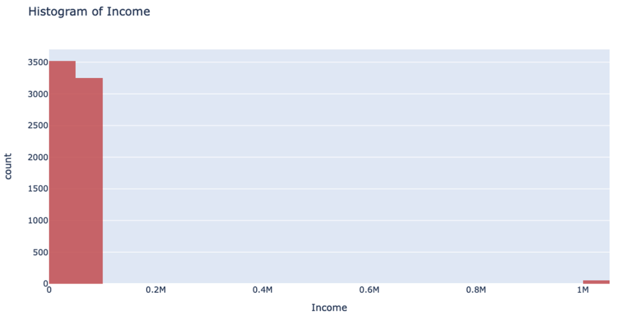
However, when you’re handling data that has a column with outliers, this isn’t the most effective way to handle your data. Suppose you’re analyzing yearly income for a neighborhood: the vast majority of the people you’re looking at are making somewhere between $20-$80k. However, there are a few outliers in the neighborhood who make well-over $1 million. When splitting the column up for binning, it will still make uniform splits regardless of the distribution of data. Because the column splitting gets skewed with large outliers, all the outlier observations are classified into a single bin while the rest of the observations end up in another single bin. This, unfortunately, leaves most of the bins unused.

This can also drastically slow your prediction calculation since you’re iterating through so many empty bins. You also sacrifice accuracy because your data loses its diversity in this uneven binning method. Uniform splitting on data with outliers is full of issues.

UniformRobust learns from previous layers to make better distributions

The introduction of the UniformRobust method for histogram  (histogram_type="UniformRobust") mitigates these issues! By learning from histograms from the previous layer, we are able to fine-tune the split points for the current layer.

The UniformRobust method isn’t impeded by outliers. It starts out using uniform range based binning. Then, it checks the distribution of the data in each bin. Many empty bins will indicate this range based binning is suboptimal, so it will iterate through all the bins and redefine them. If a bin contains no data, it’s deleted. If a bin contains too much data, then it’s split uniformly.

So, in the case that UniformRobust splitting fails (i.e. the distribution of values is still significantly skewed), the next iteration of finding splits attempts to correct the issue by repeating the procedure with new bins. This allows us to refine the promising bins recursively as we get deeper into the tree.

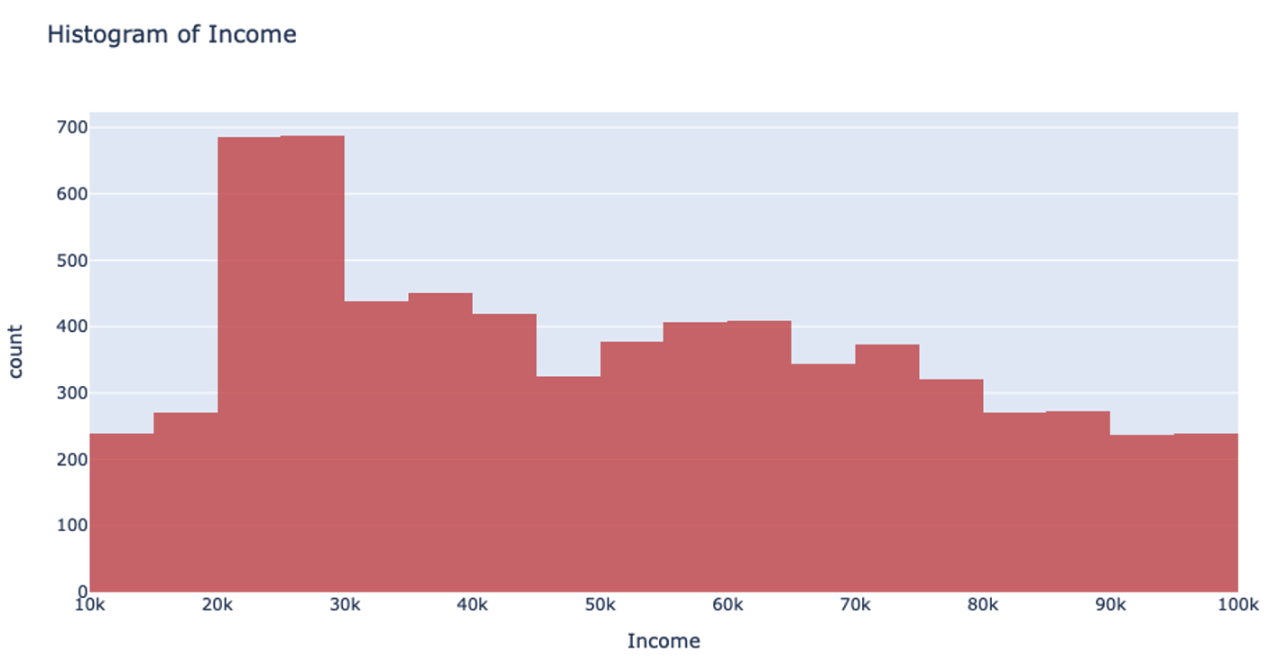
Let’s return to that income example. Using the UniformRobust method, we still begin with uniform splitting and see that very uneven distribution. However, what this method does next is to eliminate all those empty bins and split all the bins containing too much data. So, that bin that contained all the $0-100k yearly incomes is uniformly split. Then, with each iteration and each subsequent split, we will begin to see a much more even distribution of the data.

This method of splitting has the best available runtime performance and accuracy on datasets with outliers. We’re looking forward to you trying it out!

Example

In the following Python example, you can compare the performance of the UniformRobust method against the UniformAdaptive method on the Swedish motor insurance dataset. This dataset has slightly larger outliers in its Claims column.

import h2o

from h2o.estimators import H2OGradientBoostingEstimator

h2o.init()

# Import the Swedish motor insurance dataset. This dataset has larger outlier

# values in the "Claims" column:

motor = h2o.import_file("http://h2o-public-test-data.s3.amazonaws.com/smalldata/glm_test/Motor_insurance_sweden.txt")

# Set the predictors and response:

predictors = ["Payment", "Insured", "Kilometres", "Zone", "Bonus", "Make"]

response = "Claims"

# Build and train the UniformRobust model:

motor_robust = H2OGradientBoostingEstimator(histogram_type="UniformRobust", seed=1234)

motor_robust.train(x=predictors, y=response, training_frame=motor)

# Build and train the UniformAdaptive model (we will use this model to

# compare with the UniformRobust model):

motor_adaptive = H2OGradientBoostingEstimator(histogram_type="UniformAdaptive", seed=1234)

motor_adaptive.train(x=predictors, y=response, training_frame=motor)

# Compare the RMSE of the two models to see which model performed better:

print(motor_robust.rmse(), motor_adaptive.rmse())

36.03102136406947 36.69581743660738

# The RMSE is slightly lower in the UniformRobust model, showing that it performed better

# that UniformAdaptive on a dataset with outlier values!