


H2O Releases 3.40.0.1 and 3.42.0.1

Our new major releases of H2O are packed with new features and fixes! Some of the major highlights of these releases are the new Decision Tree algorithm, the added ability to grid over Infogram, an upgrade to the version of XGBoost and an improvement to its speed, the completion of the maximum likelihood dispersion parameter and its expansion to the Negative Binomial family, and many more exciting features!
Decision Tree
We implemented the new Decision Tree algorithm which is a powerful tool for classification and regression tasks. The Decision Tree algorithm creates a tree structure in which each internal node represents a test on one attribute. Each branch emerging from a node represents an outcome of the test, and each lead node represents a class label or a predicted value. The Decision Tree algorithm follows a recursive process to build the tree structure. This implementation currently only supports numeric features and a binary target variable.
Binning for Tree Building
To handle large datasets efficiently, the Decision Tree algorithm utilizes binning as a preprocessing step at each internal node. Binning involves discretizing continuous features into a finite number of bins. This reduces the computational complexity of finding the best attribute and threshold for each split. The binned features are then used for split point selection during tree construction, allowing for faster computation. The attribute and threshold combination that minimizes the weighted average of the entropies of the resulting subsets is selected as the best split point.
Entropy as a Splitting Rule
The Decision Tree algorithm employs entropy as the splitting rule to determine the best attribute and threshold for each node. Entropy measures the impurity or disorder within a set of samples. The goal is to find splits that minimize the entropy and create homogenous subsets with respect to the target variable.
The entropy of a set S with respect to a binary target variable can be calculated using the following formula:

where:
p1 is the proportion of positive (or class 1) samples in S
p0 is the proportion of negative (or class 0) samples in S
The attribute and threshold combination that minimizes the weighted average of the entropies of the resulting subsets is selected as the best split point.
GLM AIC and log likelihood implementation
We have implemented the calculation of full log likelihood and full Akaike Information Criterion (AIC) for the following Generalized Linear Models (GLM) families: Gaussian, Binomial, Quasibinomial, Fractional Binomial, Poisson, Negative Binomial, Gamma, Tweedie, and Multinomial.
The log likelihood is computed using specific formulas tailored to each GLM family, while the AIC is calculated using a common formula that utilizes the calculated log likelihood.
To manage the computational intensity of the implementation, we introduced the calc_like parameter. Setting calc_like=True, you enable the calculation of log likelihood and AIC. This computation is performed during the final scoring phase after the model has been built.
Consider the following:
For the Gaussian, Gamma, Negative Binomial, and Tweedie families, it is necessary to estimate the dispersion parameter. During initialization, the compute_p_values and remove_collinear_columns parameters are automatically set to True to facilitate the estimation process. For the Gaussian family, the dispersion_parameter_method parameter is set to "pearson" and for the Gamma, Negative Binomial, and Tweedie families, the dispersion_parameter_method is set to "ml".
The log likelihood value is not available in the cross-validation metrics. The AIC, however, is available and is calculated by the original simplified formula independent of the log likelihood.
Maximum likelihood estimation of dispersion parameter estimation for Negative Binomial GLM
We implemented negative binomial regression with dispersion parameter estimation using the maximum likelihood method for Generalized Linear Models (GLM). Regularization is not supported when using dispersion parameter estimation that uses the maximum likelihood method. To use this new feature, set the dispersion_parameter_method="ml" along with family="negativebinomial" in the GLM constructor.
Variance power and dispersion estimation for Tweedie GLM
We implemented maximum likelihood estimation for Tweedie variance power in GLM. Regularization is not supported when using the maximum likelihood method. To use this new feature, set the dispersion_parameter_method="ml" along with family="tweedie", fix_dispersion_parameter=True, and fix_tweedie_variance_power=False in the GLM constructor. Use init_dispersion_parameter to specify the dispersion parameter (ɸ) and tweedie_variance_power to specify the initial variance power to start the estimation at.
To estimate both Tweedie variance power and dispersion, set dispersion_parameter_method="ml" along with family="tweedie", fix_dispersion_parameter=False, and fix_tweedie_variance_power=False in the GLM constructor. Again, use init_dispersion_parameter to specify the dispersion parameter (ɸ) and tweedie_variance_power to specify the initial variance power to start the estimation at.
For datasets containing zeroes, the Tweedie variance power is limited to (1,2). Likelihood of the Tweedie distribution with a variance power close to 1 is multimodal, so the likelihood estimation can end up in a local optimum.
For Tweedie variance power and dispersion estimations, estimation is done using the Nelder-Mead algorithm and has similar limitations to Tweedie variance power.
If you believe the estimate is a local optimum, you might want to increase the dispersion_learning_rate. This only applies to Tweedie variance power and dispersion estimation.
Regression Influence Diagnostic
We implemented the Regression Influence Diagnostic (RID) for the Gaussian and Binomial families for GLM. This implementation finds the influence of each data row on the GLM coefficients’ values for the IRLSM solver. RID determines the coefficient change for each predictor when a data row is included and excluded in the dataset used to train the GLM model.
For the Gaussian family, we were able to calculate the exact RID. For the Binomial family, we use an approximation formula to determine the RID.
Interaction column support in CoxPH MOJO
Cox Proportional Hazards (CoxPH) MOJO now supports all interaction columns (i.e. enum to enum, num to enum, and num to num interactions).
Improved GAM tutorial
We improved the Generalized Additive Models (GAM) tutorial to make it more user-friendly by employing cognitive load theory principles. This change allows you to concentrate on a single concept for each instruction which reduces your cognitive strain and will help to improve your comprehension.
Grid over Infogram
As a continuation of the Admissible Machine Learning (ML), we implemented a simple way to train models on features ranked using Infogram. This eliminates the need to specify some threshold value.
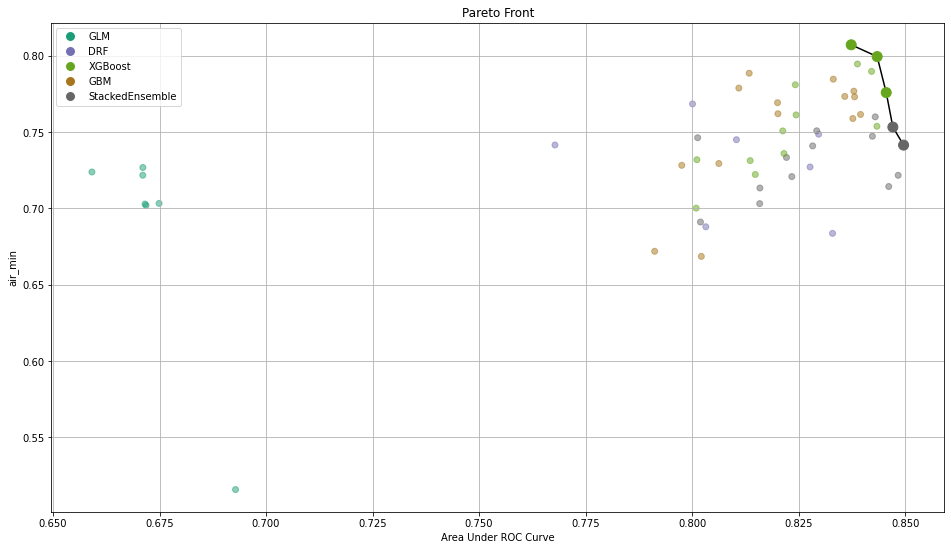
After training those models, you need a way to select the best one. To do so, we implemented the calculation of common metrics on the individual intersections. These metrics are then aggregated to form an extended leaderboard. The extended leaderboard can be used for model selection since, in cases like these, you would want to optimize by model performance and model fairness. You can use Pareto front (h2o.explanation.pareto_front / h2o.pareto_front) to do that. This command results in a plot and a subset of the leaderboard frame containing the Pareto front.
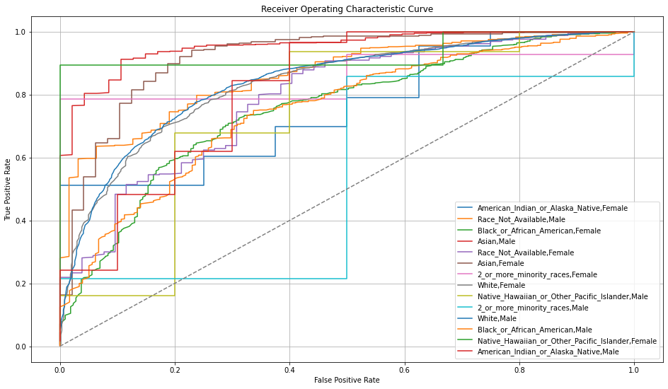
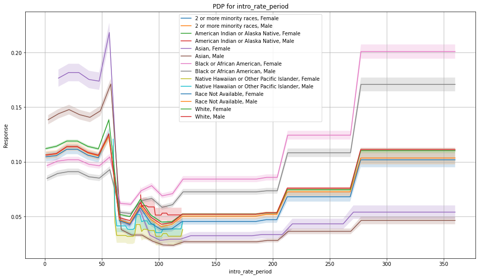
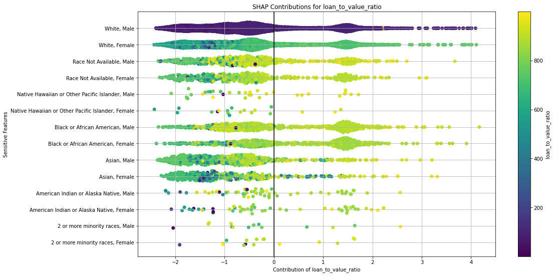
Once you pick a promising model, you can use <model_name>. inspect_model_fairness / h2o.inspect_model_fairness(<model_name>) to look at those metrics calculated on individual intersections. These include common performance metrics such as AUC, AUCPR, F1, etc., adverse impact ratio on those metrics, ROC, Precision-Recall Curve per intersection, PDP per intersection, and, if available (i.e. the model is a tree-based model), SHAP contributions per intersection. For more details, refer to the user guide.
Upgrade to XGBoost 1.6
The transition from XGBoost version 1.2 to 1.6 in the H2O-3 platform marks a major milestone in the evolution of this widely used algorithm. XGBoost, renowned for its efficiency and accuracy in handling structured datasets, has been a go-to choice for many data scientists. With the upgrade to version 1.6, H2O-3 raises the bar even further, providing users with an array of enhanced features and improvements.
One notable highlight of XGBoost 1.6 is its boosted performance, thanks to optimized algorithms and implementation. The upgrade includes various efficiency enhancements, such as improved parallelization strategies, memory management, and algorithmic tweaks. These improvements translate into faster training times and more efficient memory utilization, allowing you to process larger datasets and experiment with complex models more efficiently.
MOJO support for H2OAssembly
H2OAssembly is part of the H2O-3 API that enables you to form a pipeline of data munging operations. The new version of the class introduces the download_mojo method that converts an H2OAssembly pipeline to the MOJO2 artifact that is well-known from DriverlessAI. The conversion currently supports the following transformation stages:
H2OColSelect: selection of columns
H2OColOp: unary column operations
math functions: abs, acos, acosh, asin, asinh, atan, atanh, ceil, cos, cosh, cospi, digamma, exp, expm1, gamma, lgamma, log, log1p, log2, log10, logical_negation, sign, sin, sinh, sinpi, sqrt, tan, tanh, tanpi, trigamma, trunc, round, signif
conversion functions: ascharacter, asfactor, asnumeric, as_date
string functions: lstrip, rstrip, gsub, sub, substring, tolower, toupper, trim, strsplit, countmatches, entropy, nchar, num_valid_substrings, grep
time functions: day, dayOfWeek, hour, minute, second, week, year
H2OBinaryOp: binary column operations
arithmetic functions: __add__, __sub__, __mul__, __div__, __floordiv__, __pow__, __mod__
comparison functions: __le__, __lt__, __ge__, __gt__, __eq__, __ne__
logical functions: __and__, __or__
string functions: strdistance
GBM interpretability
We brought another insight into H2O’s Gradient Boosting Machines (GBM) algorithm. This enhancement is the ability to retrieve row-to-tree assignments directly from the algorithm. This addresses the challenge of understanding how individual data points are assigned to specific decision trees within the ensemble. This new feature allows you to gain deeper insights into the decision-making process, thus enabling greater transparency and understanding of GBM models.
GBM Poisson distribution deviance
We have updated the deviance calculation formula for the Poisson family in GBM. To ensure accurate and reliable results, we introduced a new formula:

which replaces the previously used formula:

This previous formula, though optimized and maintaining the deviance function behavior, produced incorrect output values. No longer! To validate the correctness of the new formula, we compared it with the deviance calculations in scikit-learn.
End of support for Python 2.7 and 3.5
Support for Python 2.7 and 3.5 have been removed from the project to get rid of vulnerabilities connected with the future package. If you need to use Python 2.7 to 3.5, please contact sales@h2o.ai.
Documentation improvements
Parameters for all supervised and unsupervised algorithms have been standardized, updated, and reordered to help you more easily find the information you need. Each section has been divided into algorithm-specific parameters and common parameters. GBM, DRF, XGBoost, Uplift DRF, Isolation Forest, and Extended Isolation Forest have an additional “shared tree-based algorithm parameters” section. All GLM family parameters have been centralized to the GLM page with icons showing which GLM family algorithm shares that parameter. Autoencoder for Deep Learning and HGLM for GLM also have their own parameter-specific sections.
The grid search hyperparameters have also been updated.
Contributors
Marek Novotný, Wendy Wong, Adam Valenta, Erin LeDell, Tomáš Frýda, Bartosz Krasinski, Yuliia Syzon, Sebastien Poirier, Hannah Tillman