


Summary of a Responsible Machine Learning Workflow


A paper resulting from a collaboration between H2O.AI and BLDS, LLC was recently published in a special “Machine Learning with Python” issue of the journal, Information (https://www.mdpi.com/2078-2489/11/3/137). In “A Responsible Machine Learning Workflow with Focus on Interpretable Models, Post-hoc Explanation, and Discrimination Testing,” coauthors, Navdeep Gill, Patrick Hall, Kim Montgomery, and Nicholas Schmidt compare model accuracy and fairness metrics for two types of constrained, explainable models versus their non-constrained counterparts.
Models
Explainable Neural Networks
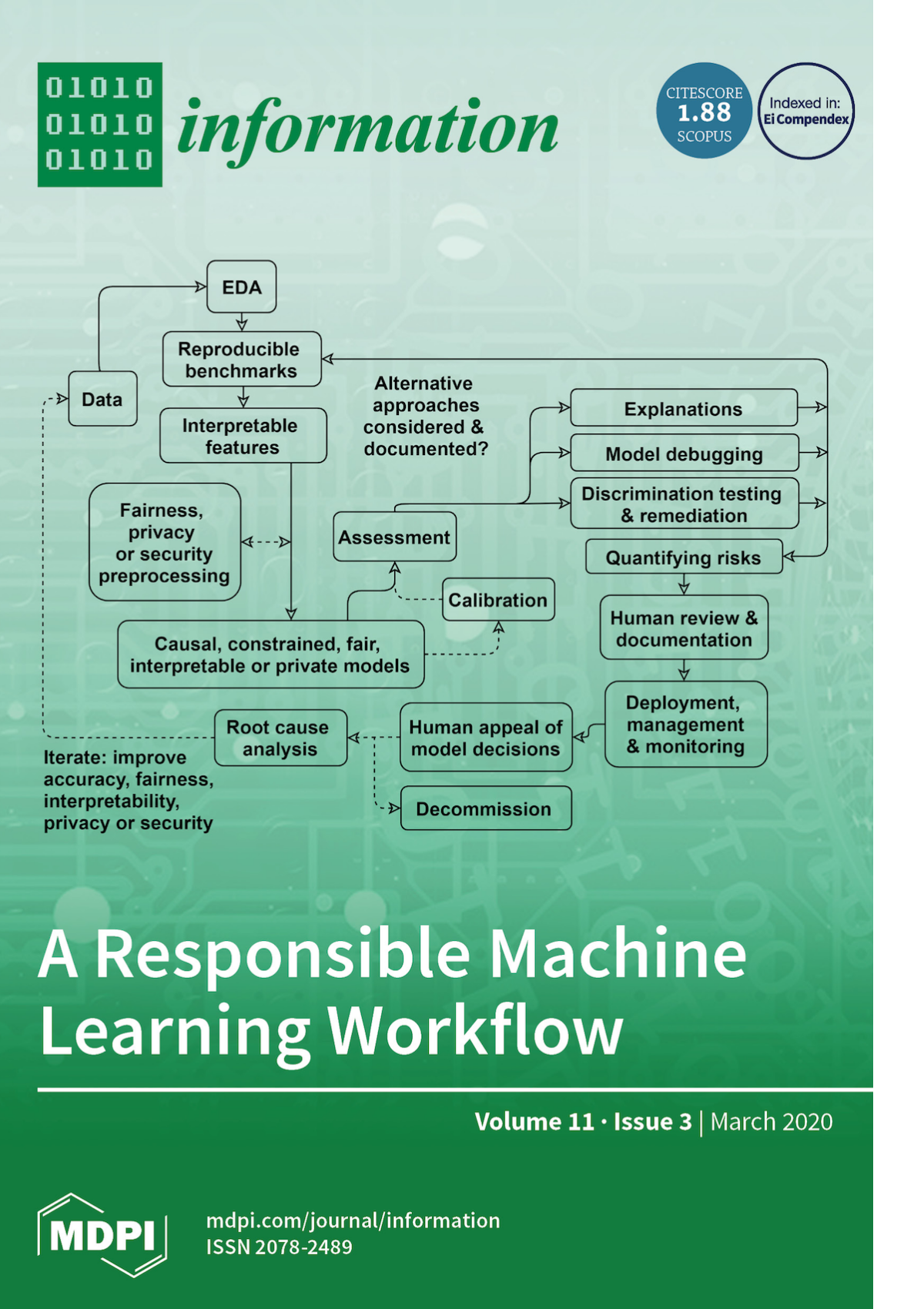
Explainable neural networks (XNN’s) are neural networks with architecture constraints that make the trained network easier to interpret [Vaughan, et. al. 2018]. The below diagram shows typical XNN architecture:
[Vaughan, et. al. 2018]
The XNN network consists of several layers. The initial projection layer calculates linear combinations of the input features. Then each linear combination of input features is fed to a separate subnetwork, h k . The subnetworks learn a nonlinear function of the projection layer outputs, referred to as the ridge function. Finally, the network calculates a linear combination of the subnetwork outputs. To promote sparsity, which increases the interpretability of the model, regularization terms were added to both the initial projection layers and the output layer.
The calculation performed by the XNN network resembles a generalized additive model,
f(x) = + 1 h 1 ( 1 T x) + 2 h 2 ( 2 T x)+… + k h k ( k T x)
except the learned nonlinear functions are functions of linear combinations of features instead of single features.
Monotonic GBM
Monotonic GBM (MGBM) is a standard gradient boosting algorithm for which the trees are constrained so that the splits in the decision trees obey user-defined monotonicity constraints with respect to the input features and the target. The monotonicity constraints were defined using domain knowledge.
Data
The models were trained on two datasets. The first was a simulated dataset produced by a known generating function based on a signal generating function proposed be Friedman.
f(x) = 10 sin( x 1 x 2 ) +20 ( x 3 – 0.5 ) 2 +10 x 4 + 5 x 5
Added to the Friedman model were two binary features and a 5 level categorical feature added for complexity, two binary class-control features for discrimination testing, and a noise term drawn from a logistic distribution.
The second dataset was a mortgage dataset taken from a set of consumer-anonymized loans from the Home Mortgage Disclosure Act (HDMA) database for which the objective was to predict whether the loans were “high-priced” compared to similar loans.
Results
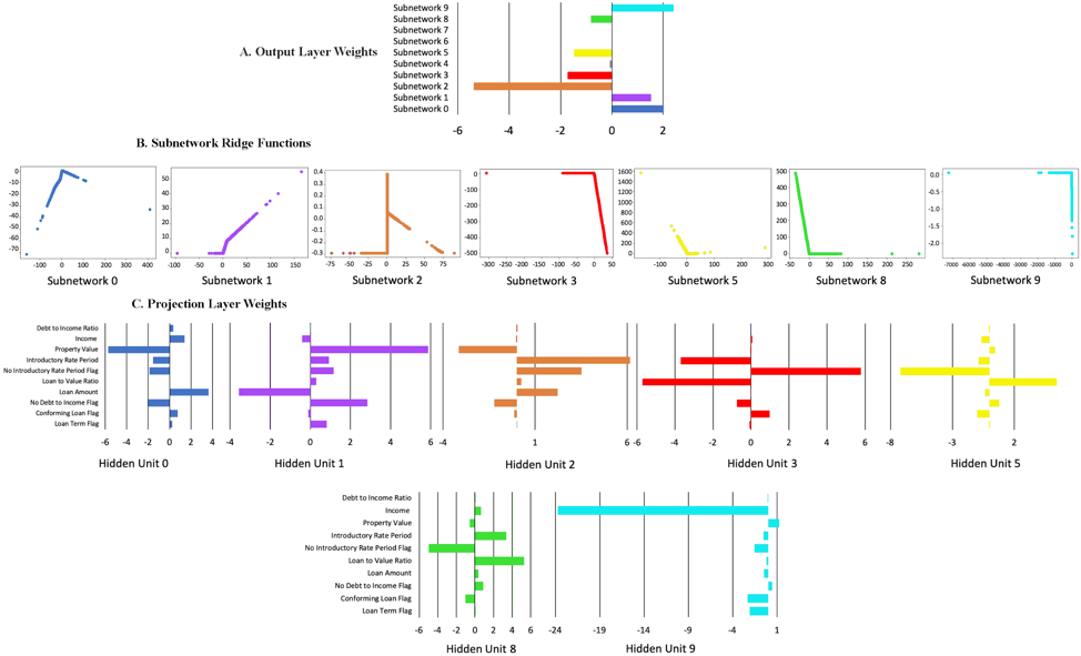
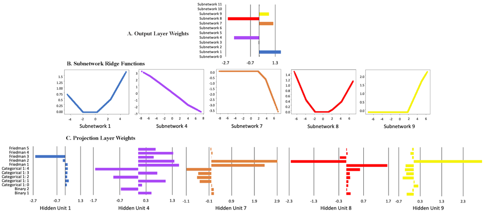
Below are the ridge functions learned by the XNN network for the simulated data. From the output weights in Figure A, only 5 of the ridge functions contributed significantly to the final result. Figure B shows the ridge functions that were learned by each of the important subnetworks. Figure C shows the weights of the original features input from the projection layer into each subnetwork.
All of the inputs to the subnetworks except for subnetwork 4 were sparse in terms of the number of original features important to the subnetwork. The input to subnetwork 1 was dominated by the Friedman x 3 function and had a shape that is roughly quadratic as would be expected. The projection layer inputs to subnetwork 4 were rather complicated, but did find the correct 2:1 ratio of the x 4 and x 5 terms from the generating equation. Subnetworks 7, 8, and 9 received inputs from Friedman functions x 1 and x 2 and reflect the network’s attempt to model the nonlinear sin( x 1 x 2 ) function which is difficult to represent due to the architectural restrictions of the network.
The ridge functions learned from the mortgage data were mostly piecewise linear functions calculated on relatively complicated combinations of the input features.
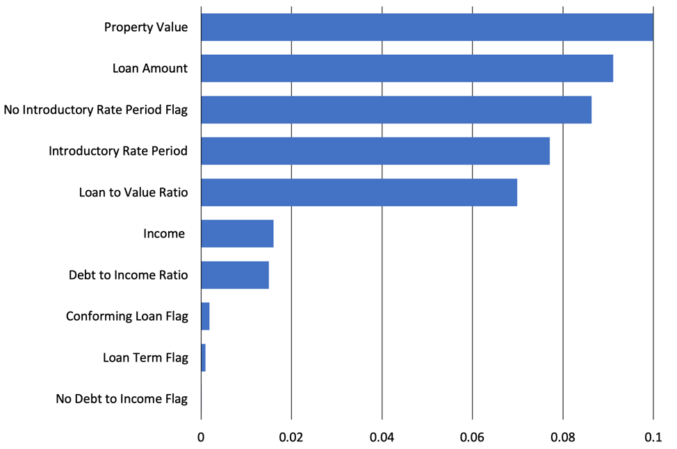
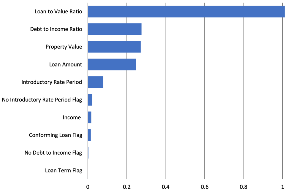
MGBM Tree Shap Feature Importance
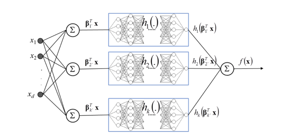
XNN Deep Shap Feature Importance
Interestingly, the Shapley feature importance for the MGBM and XNN models were quite different. For the MGBM model the loan to value ratio was most important followed by debt to income ratio, property value, and loan amount. The XNN model was less dominated by one feature and depended heavily on property value, loan amount, no introductory rate period flag, introductory rate period, and loan to value ratio. The XNN’s ability to use features more robustly may have led it to have better performance over the MGBM.
The neural network models outperformed the gradient boosting models for both the simulated data and the housing data, with the constrained XNN models producing similar results to the unconstrained artificial neural networks. The below results are from the mortgage test data. These results indicate that the XNN’s may provide a more interpretable alternative to standard neural networks for at least some problems.
| Model | Accuracy | AUC | Logloss |
|---|---|---|---|
| GBM | 0.795 | 0.828 | 0.252 |
| MGBM | 0.765 | 0.814 | 0.259 |
| ANN | 0.865 | 0.871 | 0.231 |
| XNN | 0.869 | 0.868 | 0.233 |
The below table shows fairness statistics calculated for the two restricted models. FPR is the ratio of false positives between the protected and control class where larger values indicate less fairness for the protected class. AIR is the ratio between the proportion of the protected class that receives favorable outcomes and the proportion of the control class that receives favorable outcomes. AIR values significantly below 1.0 indicate a model is less fair toward the protected class.
| Model | Protected Class | Control Class | AIR | FPR Ratio |
|---|---|---|---|---|
| MGBM | Black | White | 0.776 | 2.10 |
| Female | Male | 0.948 | 1.15 | |
| XNN | Black | White | 0.743 | 2.45 |
| Female | Male | 0.955 | 1.21 |
In the racial category, the XNN model had somewhat weaker fairness results, while in the gender category the results were quite similar. It’s not clear that either of the restricted models would help would affect fairness in general.
Conclusion
The paper presents an approach to training explainable models and testing their accuracy and fairness and tests that approach on both simulated data and a more realistic set of mortgage data. In the examples studied in the paper, the neural network models outperformed the gradient boosting models and the XNN’s were able to provide some interpretability advantages with little or no loss in model accuracy.