Responsible Machine Learning with H2O Driverless AI

Watch Webinar Replay Below

Read the Full Transcript

Patrick Moran: Hello, and welcome everyone. Thank you for joining us today for a webinar titled Responsible Machine Learning with H2O Driverless AI. My name is Patrick Moran, and I’m on the marketing team here at H2O.ai. I’d love to start off by introducing our speaker.

Navdeep Gill is a senior data scientist and software engineer at H2O.ai, where he focuses mainly on machine learning interpretability, and previously focused on GPU-accelerated machine learning, automated machine learning, and the core at H2O 3 platform.

Prior to joining H2O.ai, Navdeep worked at Cisco, focusing on data science and software development. Before that, Navdeep was a researcher/analyst in several neuroscience labs at the following institutions: CSU East Bay, UC San Francisco, and the Smith-Kettlewell Eye Research Institute. Navdeep graduated from CSU East Bay with an MS in computational statistics, and a BS in statistics, and a BA in psychology.

Before I hand it over to Navdeep, I’d like to go over the following housekeeping items. Please feel free to send us your questions throughout the session via the questions tab. We’ll be happy to answer them towards the end of the webinar. And this webinar is being recorded. A copy of the webinar recording and slide deck will be made available after the presentation is over. And without further ado, take it away Navdeep.

Navdeep Gill: Thanks, Patrick. Like Patrick mentioned, the title of the talk here is Responsible Machine Learning with H2O Driverless AI. Before we begin, I’d like to give some background about this presentation and what we’ll be talking about. Transparency, accountability, and trustworthiness are a big part of a lot of regulated industries today, whether it be banking, insurance, healthcare, or other industries. A lot of this should also be accounted for in other industries as well, like IoT, of if you work at a startup or anything like that, because if you can’t really trust the machine learning models, then you can’t really deploy them out into the real world. Being responsible in this aspect is very important for a lot of data scientists.

The problem statement we’re trying to figure out today is can the productivity and accuracy advantages of automated machine learning—can they be leveraged in highly-regulated spaces? I would like to mention that we at H2O cannot really provide compliance advice in this manner, but we like to think that these tools can be used in a very responsible manner, and you can get a lot of output from these types of tools.

And I want to talk about AutoML, and I’m specifically talking about H2O Driverless AI, which is a system that does auto visualization, automatic feature engineering, trains models, and explains models with minimal user input. The idea here is this tool can be used to work on many use cases for your business, and you can work on them in a more productive manner without having to worry about model tuning or manual feature engineering. A lot of the stuff can be automated for you with Driverless AI.

With that background information, I’d like to go over the agenda that we’ll be focusing on today. I’ll be going over these four things—an intro about explainability and responsible machine learning, why this concept matters, what you can do as a user to have more of a human-centered responsible machine learning approach with Driverless AI, and how you can explain models with Driverless AI.

Here’s the intro. First off, we have to go over some terminology that will be used throughout the presentation. The first term is machine learning interpretability. It’s the ability to explain or present in understandable terms to a human. By machine learning interpretability, you should be able to take an output of a model and explain it to business users, analysts, stakeholders, and explain to them why a certain decision was made. This is highly important for regulated industries, but it should also be accounted for in other industries as well, as you need to establish a level of trust and understanding with the machine learning models that you’re deploying.

Now Auto ML will be referenced throughout this presentation. By this, I specifically mean H2O Driverless AI. I mentioned earlier, this is an Auto ML type of tool, which Auto ML makes a lot of processes into data times workflow. As I mention Auto ML, I am referring to H2O Driverless AI.

And of course I’ll reference something called an MLI module, or MLI in this case. And by this, I mean the MLI module and the H2O Driverless AI. Driverless AI has a component that does machine learning interpretability, so when I reference MLI, I am referring to this component.

Now, we will go over a type of pipeline someone will go through in their machine learning endeavors. It starts off with data integration and quality. We know once you have your data set prepped and ready, you cleaned it up, dealt with missing values, dealt with duplicate rows, anything like that that you would typically do. Then you would move on to feature engineering, model training, and before you deploy the model, you kind of want to interpret the model to see what it’s doing.

Here are some applications we have in Driverless AI that I’ll go over later on, so you know from MLI, you would do this like disparate impact testing. This is to make sure that different groups of people or observations are treated fairly with the model. You can do what if or sensitivity analysis with Driverless AI, so this has to do with model debugging, and seeing what happens when you change an input to the model and how the output changes.

With Driverless AI, you can look at things like feature importance, you can get reason codes, which is from Shapley & LIME. You can use surrogate models to figure out how the model is behaving itself with maybe a more simpler model. You can look at things like partial dependence and ICE, which has to do with how the models output changes as you change certain inputs. Of course, the final step of this is model documentation, which most people are probably familiar with, especially if you’re in banking, insurance, or healthcare. You have to document what the model did, what sort of inputs it used, and the distribution of the training data set versus the validation on the test. This is what we call AutoDoc in Driverless AI, and this is available to all users as well.

Now, in terms of the pipeline itself, you can imagine that the feature engineering in the model training could be highly complex, and this might make the MLI aspect a little more complicated to use. And of course, the MLI aspect does not have to always be at the end. With Driverless AI, you can have MLI as the entire pipeline, so you can have interpretability in mind throughout the entire pipeline. You can constrain certain interactions with the feature engineering, and you can build interpretable models. These are things like monotonic UBMs or a generalized linear model. All of this can be limited in the scope of Driverless AI to avoid highly complex models if that is what you are concerned with getting.

Like I mentioned before, you can build a very accurate model and then interpret that accurate model and try to get some insights, or you can have interpretability in mind throughout the entire process. This is available in Driverless AI. This is something you can do today.

The next topic is why does responsible ML matter? The first thing to keep in mind is sometimes there is a potential trade-off between performance and interpretability. You can have white box models, which are models that are highly interpretable. And you can have black box models, which are very complex. It’s like a simple decision tree versus a very complicated neuro network.

When I say there’s a potential trade-off, I mean there might be a potential trade-off between accuracy. Work has been done lately that shows that you can get very highly accurate models that are also interpretable. But sometimes there still is this trade-off that can happen between two.

Also, when you have explainable models or models that are highly interpretable, you can get exact explanations for approximate models. And if you have a very complicated model, you can get approximate explanations for exact models. Imagine if I built a very complicated neuro network, I can get approximate explanations for that complicated neuro network using things like LIME, however I can also get exact explanations for that model as well using something like Shapley, for example.

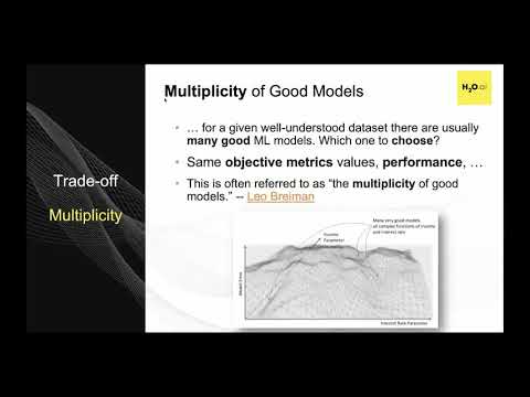
Another thing to consider with this console of machine learning is this concept of multiplicity and good models. For a well understood data set, there might usually be one best linear model. However, there might be many good machine learning models that are not linearly-based, like GBMs or known networks, so which one do you actually choose?

This concept itself is from Leo Breiman. For a given data set, you can have many models that work, and you yourself as a user have to figure out which model to use and use certain objectives to figure that out.

One objective you can use is to decide which model is more fair. You can build several highly complex models and pick a model that is the most fair to your training data set or the most set to observations, meaning a training data set. Now, fairness and social aspects are very important, especially in regulated industries. You don’t want a machine learning model that is bias based on gender, age, ethnicity, health or sexual orientation. You want to make sure that everyone’s treated equally for the groups that you’re interested in.

Another reason that responsible machine learning matters is that you want to have trust the model producers and the consumers. You might want to think about your data set versus the real world; you want to ensure that the data set you used to train the model can be well-represented from the real world. And you also want to make sure that your machine learning model itself will not go haywire in the real world if it sees something that’s it never saw during training, so you want to account for this during your training process. You want to have some type of introspection into your machine learning model. You want to understand how sensitive this machine learning model is before you deploy it, whether that be through diagnostics or model debugging, which I will go over in later slides.

But you know, a lot of these things should not only be accounted for in regulated industries. They should be accounted for in probably every machine learning application before you actually go out and deploy something that’s going to make automated decisions for you.

Another thing with responsible ML to consider is this concept of security and hacking. Sometimes a model can be deployed, and it can be hacked. There have been studies that have shown that it’s possible if the model is available through a certain API, someone can use, let’s say, a surrogate model, which will be trained on the predictions of your model, and figure out what the inputs were. And based off that, build out data sets that represent the training data that’s used for your model itself. And you can avoid these types of things by using adversary data sets or adversary instances. Try to figure out how you can change the outcome of your model from being one to zero, or vice versa, based on certain changes in your data set itself. You can look at the integrity of the model, so this has to do with false negative instances, fraud path checking. You can also look at your false positive instances. A lot of these things can be explored before the model is deployed to ensure that security and hacking are not a threat to you.

Also, another thing to consider with responsible ML is in many industries that use machine learning, they are also regulated themselves. There are legal requirements about ensuring that you’re using machine learning responsibly, whether it be banking, insurance, or healthcare. You have to justify the decision that is made for an observation. This is usually through something called reason codes or adverse action notices. Adverse action notices are using banking heavily, and this has to do with if someone is denied a loan or credit, you have to explain to them why they were denied a loan or credit line.

If you’re able to do this adequately, then you’re protecting your business and yourself from any adverse effects from deploying a machine learning model that did not make sense or people did not understand.

In summary, the reason that responsible machine learning matters is that you want to have a balance between performance and interpretability. You want to think about the multiplicity of good models, so you should not only choose models based on accuracy, or AUC, or any type of metric. Keep in mind the model’s fairness and how interpretable the model is. You want to take into account fairness and social aspects. You want to have some trust in your model itself. You want to keep track of security and hacking of your machine learning model. And of course, if you’re in a regulated industry, you want to keep those regulations in mind.

Now we’ll talk about what’s needed to build out this human-centered responsible machine learning with Driverless AI. The first step with Driverless AI or a lot of machine learning applications is you know you want to load your data. With Driverless AI, you can load your data, and you can instantly get some exploratory data analysis of the data set loaded. This is the first step in responsible machine learning—ensuring that the data you have is cleaned up, it makes sense to you based off of your domain knowledge, it makes sense maybe to other team members that you work with so they understand that the data used is representative of where this model will be deployed. Driverless AI gives that to you out of the box as the data set is loaded in.

Once your data set is loaded in, we have this concept of auto visualization. This is worked on by Leland Wilkinson, who’s very well known for the grammar of graphics. And what this module does is, once a data set is loaded in, you can visualize the data set, and the auto visualization will figure out interesting characteristics about the data set and present that information to you. This is really nice, because you don’t have to do it manually. And you’re taking the first step in responsible machine learning in an automated fashion, and you can iterate very quickly through these plots, figure out if there’s anything that doesn’t make sense, and if it doesn’t make sense, you can go on to the next step.

These are the types of plots you can get. You can look at correlations, and you can look at outliers. These are the type of things that are a part of the pipeline with the human-centered approach.

The next step feature engineering. Like I mentioned before, in Driverless AI, we offer automated feature engineering. The features themselves can vary in complexity. Depending upon what your goal is, if your goal is to have an interpretable model, you can play with this interpretability knob that you can see highlighted here. In this case, when we turn the interpretability knob down to one, this will produce a lot of features with varying complexity. If this is your goal or this is something you can deal with, then you can set interpretability for this level.

However, if you wanted a white box model or a white box type of feature engineering, you can turn interpretability all the way up to, let’s say, 10. This will make features that are highly interpretable, people can understand them, and the explanations for these features makes sense. Depending upon what your goal is, you can go this route as well. From a responsible machine learning standpoint or an interpretable machine learning standpoint, you probably want the interpretability to be a little higher than one, so you can avoid any misunderstandings with the features you use.

Here I have a few figures here that I can show in Driverless AI later on as well. But essentially what these two figures are showing is—on the top one there, figure one, I am setting the reproducibility on Driverless AI. I can get reproducible results, which is very important for machine learning. Also, I am setting the interpretability to seven, and this will give me feature engineering that’s pretty interpretable for more people. These are features that you can present to business users or to analysts on your team that aren’t probably advanced data scientists, but you can explain to them what this feature is and they will understand it.

Setting this interpretability to seven also adds monotonicity constraints. Basically, as the input feature volume increases, the output of the model can only increase, or vice versa. This is something you can control with Driverless AI. This is something you can constrain the model itself to do.

Another thing you can do is set which models to use and which models not to use in Driverless AI, which is shown in figure two. You can see there that I’ve turned basically everything off except for XGBoost and GBM, and the things monitoring the constraints are on. This is a pretty accurate model that is modeling relationships in a monotonic way. The inputs and outputs would make sense to someone, and this is something you can do before you even start your Driverless AI experiment.

Once you’ve loaded your data in, you’ve made sure that there’s nothing funny going on, and you’ve done some exploratory data analysis using the auto visualization module of Driverless AI. You’ve done feature engineering, and you’ve figured out what type of feature engineering you want, whether it be like a white box type of feature engineering or a black box type of feature engineering. Then the next step is to actually build out the models.

Now, the type of model you want depends upon what your end goal is, but if your end goal is interpretability, then you want to build out these white box models, these models that make sense to people—these models that probably won’t build out too many crazy interactions that are hard to comprehend.

You can do this just by setting interpretability in Driverless AI to, let’s say, 10, accuracy six, and then time is four here. You can see I have monotonicity on again. I’m using the tree-based models, and I’m using feature engineering, like frequency encoding, one hot encoding, and looking for a time variable. These are features that people will understand, and these are features that are actually being produced by Driverless AI, so it’s no work on your part. The system is taking over and building these out for you.

You can see here that this is a breakdown of the what the interpretability knob can do. So you know if you have interpretability set to one and three, it will do a lot of feature engineering; it can build out ensembles. You can see as I increased the interpretability up to four, or five, six to 10, the ensemble level goes down, meaning my final model will be a single model or a small amount of models instead of a huge ensemble. The target transformations are going away at that point where the target remains and it’s no more space; the feature engineering itself is getting a little more interpretable.

Here are some of the screenshots that you see in Driverless AI. So here, for example, I’m setting GLM models to on.

Let’s go back over the models again. Driverless AI offers many interpretable models. We have GLMs, we have RuleFit, and then I mentioned monotonicity earlier, so one that’s enabled—all the tree-based models are essentially monotonic GBMs. By default, Driverless AI will use an ensemble with several types of models, which can be undesirable from an interpretability perspective. However, you can change this to build no ensembles at all, which would probably play in your favor from an interpretability standpoint.

For example, down here again you can see that I have turned off all models except for the XGBoost and GBM, and I’ve set the ensemble level to one here, which would mean only a single model will be built at the end instead of an ensemble of models. This is going back again between balancing accuracy versus interpretability. If I built in a huge complicated ensemble, it might be really accurate compared to a single model, because interpreting it might be quite difficult. This is a balancing act you can play with Driverless AI, and you can run many experiments this way and compare results, and then at the end, pick the one that makes the most sense to you and your use case.

Another thing we offer in Driverless AI is this mode called compliant mode. What compliant mode means is it will force the interpretability knob to be 10. The type of model we will use will be GLM or RuleFit, treating certain features like neuro features as categorical. It won’t use any ensembles. The interactions are not too deep for these type of models. The target transformed is pretty much turned off. And it won’t even need distribution shifts between train, valid, and test to drop features.

Essentially, this type of load will do what I spoke about previously in one shot. I can turn the compliant mode on and it will set everything to these bullet points you see here, instead of having to do it one by one.

Again, I was talking about compliant mode. This is a way to ensure that simple models are built—simple feature transformations are done in a one-click shot.

Once the model is built, the next step in this type of pipeline is the assessment of the model itself. Looking at things like the ROC curve, lifts, gains, the K-S charts—all of these are built into Driverless AI. You can get these out of the box. There is not any manual work needed on your part. All this information is available to you once the experiment is done.

Another thing we offer, which I mentioned in a previous slide, is this concept of AutoDoc. This is a Word doc that goes over everything that was done in the experiment. This is highly important in regulated industries, but it’s also important in any industry that uses machine learning, because you want to be able to explain to people what you did with your machine learning model and how you built it. This is nice in the sense that you don’t have to do it yourself. It’s done automatically for you. All this information is available to you at the end of the experiment, and you can distribute it to your team or to various stakeholders.

Once again, in addition to the assessment that’s done after the experiment, you can also run diagnostics of your model on the different data sets, and then, this is how you can compare models on various test sets. Let’s say you have model A and B: you can compare its performance on the test set, and you can get an output like this under the diagnostics tab of Driverless AI.

Once you’ve built the model, and you’ve done the assessment, then you would move onto to this MLI component, which shows the “what if” sensitivity analysis. You’re reading codes and disparate impact testing.

Once the experiment’s over, you can type in enter, or you can click on interpret this model, and then all of this stuff will be launched for you, and then the results will be available as well in the form of a dashboard in the MLI pane. And then the other tab will show each chart specifically.

Once you’ve gone to this point, the next step is the human review component, which making sure that the results you’re seeing make sense to your use case. You look at local instances, reason codes, adverse action notices, local instances, and model debugging. Global instances of feature importance is where you look at the documentation and look at the performance of the model itself. This is where the human review comes in. But the beauty of Driverless AI is that you can iterate very quickly, and you can jump to human review very quickly, and you can compare various models across diagnostics, across MLI, across accuracy and performance, and you can tackle many use cases this way.

The next step is how we go about explaining the output. If you recall, we’re still talking about responsible machine learning. A big component of that is figuring out what your model did and ensuring that you are not introducing any bias to the output itself.

This is more of a deep dive into the MLI module. Once you’re in Driverless AI and you click on “interpret this model,” you will get a dashboard like this, among various other things. I’ll do a deep dive into that. The main focus of this talk is on IID data, so this is not like time series data or MLP type data; this is a normal tabular datasets. That’s the focus of these next few examples and slides that I will be showing.

The Driverless AI module can be broken down into this type of flow. We have this global approximate model of behavior interactions. This is usually done through a concept known as a surrogate model. We offer various kinds of these in the MLI module itself. You can look at global feature importance. These are things like Shapley values from a global manner, and the model’s feature importance. RF stands for Random Forests, which is a surrogate model that we built, and you can look at the feature importance of this surrogate model itself.

You can look at global feature behavior, which is PDP or Partial Dependence Plot. On average, this shows how the output changes if I change all the rows to a certain input. That’s the concept of PDP. You can get reason codes as well. This is done through LIME, or we call it K-LIME. .I’ll go over this concept later on, but essentially this is building a linear surrogate model to the output of your Driverless AI model, and then building reason codes, which are essentially coefficients of the GLM model. Then, based off of that, you can get global reason codes and local reason codes as well.

Driverless AI offers Shapley values for a lot of its tree-based models. These aren’t really approximate reason codes—these are the actual reason codes used by the Driverless AI model.

So again, all of this material that I just went over is done on a global scale. You can also do it on a local scale. By local, I mean looking at rows or groups of rows. This is all available in the MLI module today.

Later on, I’ll be showing a few experiments done in Driverless AI, and this is the dataset we’ll be using. It’s a credit card data set; ;the features itself that are used are things like limit balance, so that’s the amount of credit given to a user. We have information about their gender. It won’t be used in the model, but we have this information to check for disparate impact later on. We have the education levels, which won’t be used in the model again, but we can check for disparate impact later on. We have their marital status, their age, their repayment statuses, the amount they were billed, and the amount they paid for the previous month. This is the dataset that will be referenced later on in the experiments that I show, and I just wanted to go over it now so people understand the type of features that you’ll be looking at. And of course, I’ll go over these features as we’re looking at the experiment.

The first thing we can look at in Driverless AI is this global approximation to model behavior and interaction. The challenge here is that you have some black box model, and you’re trying to understand how it made certain decisions. One thing you can do is build a surrogate model for this. Now, what is a surrogate model? A surrogate model is a maybe a simpler model—imagine a decision tree with a single tree that’s built to the output of the complicated model. This is building a decision tree to the Y hat or the prediction of the Driverless AI model. And then based off that, you can plot that single tree and you can see how certain decisions are made, so you get this model flow of what happens. Those are the pros to this type of approach.

Since it’s a simple model, which in this case is a single decision tree (which is what we offer in MLI), the con can be the accuracy. The good thing is that you get a flow of what’s going on. However, keep in mind that if the accuracy is pretty low, then it’s not capturing all the variants from those predictions. But if it is pretty accurate, this is a very good way to figure out what’s going on with the complicated model from a visual depiction standpoint.

This is what I was just talking about earlier. How are surrogate models made? Here, I’ve built a model with my own matrix of X features, my output Y. And the surrogate model is those same features, but built to a Y hat, which is the prediction of the previous model itself. This is how you would go about building a surrogate model. Based on this, you can use a lot of things to build surrogate models. You can think of GLM and build a surrogate model for a complicated GBM, for example.

Another thing we can look at is the global feature importance, so this is the typical feature importance you would get from any machine learning model. You can look at this feature importance from a surrogate model as well. In MLI, we built a random force surrogate model to the Driverless AI prediction, and then we plot the feature importance of the original features used in that experiment. Based on this, you can get some introspection into what the model thinks is important. That’s the pro again, but the con is the accuracy, so you have to keep in mind if the surrogate model is accurate to your Driverless AI model.

We provide metrics in the MLI module to let you know how accurate it is, and based off those metrics, you can see if you trust the important plot itself.

Another thing we offer is the feature importance of the original model itself, so you can look at the surrogate model feature importance and the original model feature importance, and you can compare and contrast the two to see how much a surrogate model is capturing from your model itself. This goes back to the whole security thing. If your surrogate model can capture a lot of variants of the output of your Driverless AI prediction, the same can happen if let’s say a hacker tried to get into your model itself. They can probably build a surrogate model to capture that variant as well. So it’s something for you to keep in mind and another application of surrogate models.

Another thing we offer is a Shapley values, which I’ll explain in the next slide. But essentially this is a very robust way of getting feature importance. It’s been tested a lot in literature. There’s that whole packet behind it. That’s the pro of this approach. The con is it can take a long time to run Shapley values. And we offer it for transformed feature currently, so we are working on a way to get Shapley values for original features.

Here’s a breakdown of Shapley values, which I mentioned I will go over. The inventor of this concept is Lloyd Shapley. He won a Nobel prize for this work in 2012. Shapley values itself come from game series. Like I mentioned before, it’s a highly complex calculation, so you know it adds a lot of time complexity, exponential time complexity. It’s unrealistic to compute in the real world. You can compute it on a global scope, which is what I showed previously, but also you can take that same complexity to a local scope, which is for a row or a group of rows.

The idea behind the Shapley value in simple terms is it comes from game theory, and the idea is there’s a group of people playing a game, and there’s some payout. How can I equally distribute the payout amongst the people in the game? Or how can I distribute the payout amongst the people in the game? That same concept can be applied to features and the output is the prediction of the model. How are the features distributing amongst the output, amongst the outcome of the model itself? And that’s where Shapley values come into play for machine learning.

The traditional approach is highly complex, but there is the work done with Shapley values on tree-based models, which is what we use in Driverless AI, and that work has shown it can be done pretty quickly, and the time complexity goes away or almost goes away with that approach.

Another concept of feature importance that we offer is to leave one covariate out. The idea here is, with our random force surrogate model, if I set one of the features to this thing, and then I rescore that model, how does the outcome change? That is what we do with this concept of leaving one covariate out.

This is another way of looking at defined feature importance, just like the Shapley plot itself. So you have various ways of looking at the importance of variables and comparing and contrasting how they’re different with different approaches. This is like a matrix view of how leaving one covariate out would work.

We’ve gone over the random force surrogate model, leaving one covariate out, thinking of feature importance of the original model, and the Shapley value itself.

The next concept is partial dependency. The concept here is looking at the average output of the model as you change the entire set of rows to a certain value. This gives you the distribution of the prediction from a global scale. And this is what we offer in MLI as well. So if I have a variable Xj, and I set that to one constant value, then I score the model and get the average and the standard deviation, I can plot those and see how the outcome changes, based off of setting that Xj to certain values.

Here are some examples. The PDP can be flat. Not much is changing with the model outcome as I vary the feature itself, so maybe this is something you can look at from a local scale. You can also look at the PDP, like the bottom one there where it shows a spike, and then it levels off. All of this is just basically going over the behavior of the model from a global scale, and based off of your domain expertise or what you know about the data set, you can verify if this makes sense or not.

The next step is looking at local feature importance on MRI. We have this fast forward where we have something like a K-LIME plot. We have feature importance. We have PDP, and we have the decision tree surrogate model. This is all shown at a global scale initially, but you can zoom into a row, and you can see the reason code for that row, the feature importance for that row, what path it went down, and the decision tree surrogate model, and the conflict of ICE, which is the same as PDP, but just done for a single row of data.

In this case, you see highlighted here the reason codes for the K-LIME plot, the plot left there. This helps with debugging and drilling down from a global to local scope. The surrogate method used here is K-LIME, which I will go over in later slides as well.

There’s this concept of LIME, which is used for getting local reason codes. The idea here is that I have some row of data, and then I sample around that row of data to build out similar rows, and then I build a GLM to those rows, and get reason codes. This is something that been shown in literature with the LIME package. However, it can take a lot of time to build out the sampling approach. Here you can see there’s a row, which is indicated by the plus sign. I sample around that row to build out a data set, then I build a GLM, and then I get reason codes for that row.

What we do with the MLI module is we do this concept called K-LIME, so instead of sampling around specific rows, what we do is we build first through k-means to cluster the data, and then for each cluster, we build a generalized linear model, which can be used to get reason codes for rows that fall within that cluster. This is a much faster approach than sampling, which can take quite some time.

And then based off of selecting the row in the K-LIME plot, which shows here, we selected a row, it belongs to cluster two, we can see where the feature importance for that row, we can see its ICE plot on the bottom right there, so comparing that to the PDP plot, we can see what path we went down in the decision tree model itself. Once again, this helps with drilling down to what’s happening for specific rows, and also helps with debugging as well.

Another thing we offer with K-LIME is you can get reason codes for a specific row. Here, you can see there’s an explanations button. I can click on that explanations button, and then get English written reason codes to understand why a certain prediction was made for the model itself.

Here you can look at the decision tree surrogate model, and what path this row went down to understand the reasoning behind the prediction itself from a local perspective.

Again, we also offer local feature importances for the random forest (RF) surrogate model and for the Leave One Covariate Out (LOCO). We offer it for Shapley as well.

One thing to keep in mind that I mentioned earlier, is that with local feature importance, you can get this concept of adverse action notices. An adverse action notice is a set of reasons to explain why a lender or employer has taken some negative action on someone. If machine learning is used to make these decisions, then generally these adverse action notices are very important. In the dataset we’re using, it’s the credit card data set, and we’re predicting if a person will default on their next payment or not. In this case, we want to understand why a certain reason was made just in case someone asks why they were denied. We need to have some solid reasoning behind why a decision was made. And if we’re using machine learning models and we’re doing it in an automated fashion, we have to make sure that those reason codes make sense. This is something we offer through the MLI module itself with various methods like the local feature importance, Shapley values, K-LIME reason codes, and various surrogate models that you can look at as well.

Using all this information together, you can figure out why certain decisions were made, and then based off that you can debug you can see if it makes sense or not.

This is just like a plot of the Shapley values for a local row, and you can see here what’s important and what’s not important as well for this specific row, compared to the global case.

Another thing we offer is this concept of ICE. ICE is individual conditional expectation. The concept here is running PDP for a specific row, so you can look at everything on a single plot; those yellow dots there is the global PDP. The gray plot is for a specific row, and that dashed line is the model prediction itself. Based off this, you can look at the distribution of the model outcome on average, and you can look at the distribution for a specific row and then compare that to what the actual score was.

We also offer in Driverless AI auto documentation. This is a way of seeing how the experiment played out in Driverless AI. Seeing PDPs, again, in this case you can look at out-of-range PDP, so seeing how the model is behaving when it sees data that it did not see in training. This goes into the sensitivity of the model itself. Once you have this auto documentation, this is something you can go over, and this is the human review aspect that comes into play. The MLI module itself also offers the ability to download all the images, so these can be shared amongst team members or other people in your company or organization. And this is also a good way to get feedback from your experiment. Since Driverless AI is an automated system, you can do this with various experiments and share the results with the pertinent people.

Let’s go over the model documentation again. One thing we are offering in the next release of Driverless AI is a disparate impact analysis, so this is a way to look at various metrics across groups to see if there is any disparate impact. Disparate impact means that there is unfair treatment of certain protected groups. For example, if you built a model that was predicting defaulting on a loan, and in the model itself you did not use a gender variable, that’s not to say that disparate impact wasn’t completely avoided. There could be a fair or an unfair treatment between males and females, so you can look at that with the disparate impact tool in the MLI module itself.

The last thing we offer is “what-if” and sensitivity analysis. They’re a validation technique. The idea here is basically you want to take the inputs and change them, and then see how the outputs are changing. This is a very good way to do model debugging, and a very good way to figure out if there’s any interesting behavior going on with the model itself. The you can address then that behavior before it’s deployed.

This is a new concept that we will have in the next release of Driverless AI in the MLI module.

With that, I can open the floor for questions.

Patrick Moran: All right, thanks Navdeep. As these questions start rolling in, I just want to remind everybody that we offer a 21-day free trial of Driverless AI. You can access that from our website. I will provide a link in the attachments post webinar as well, but the website is H2O.ai/try. That’s a quick way to get to the signup page to request a free trial license. And it’s a great way to just get your hands on an automatic machine learning platform and start playing around with MLI as it pertains to your business use case.

Navdeep Gill: I can jump right into Driverless AI, so like Patrick mentioned, you can get your hands on a 21-day trial. I’ll just quickly go over some of the concepts and some of the presentation, and show you in the software itself. In this case, I uploaded a dataset, which you can get from your file system, S3, Hadoop, a URL, or you can just upload it directly from your own computer if you have Driverless AI running on an instance or anything like that.

In this case, I uploaded the two datasets. There’s a train set and a test set. And one thing you can do with Driverless AI is you can click on the dataset and look at the details. This is going over distribution and the breakdown for categorical variables, and the breakdown for continuous variables. You get many characteristics like the count, number missing, mean, median, and mode. This is something that goes into the initial aspects of the VDA itself. Once you’ve done that, you can visualize a data set. I’ve already ran this, but initially, we just click on the data set and then click on visualize. Here you can go to auto vis. We’ve got the training data set. These are all the visualizations that have been made, and these are automated insights that are made from the auto vis module itself. We can look at things like correlation plots, which in this case are the bill amount, and bill amount two. You can look at the help section, which gives you an English explanation of what you’re seeing, and you can download the plot itself. This is available for all data sets that are imported, and this is a very good initial set in any data science pipeline.

I mentioned before that once you’ve done auto vis, you can go into an experiment. What I was mentioning earlier is that you can click on the dataset you want to use. If you don’t want to use protected groups in your experiment itself to avoid any bias, that is not to say it will completely avoid bias, but this is a good first step. In this case, we’re trying to predict if the person will default next month on their credit card payment.

I was mentioning earlier that you can go into the expert settings for the experiment itself. You can select which models to use. Here I can use XGBoost but turn off everything else, for example. And then I can use the ensemble level; if I set that to zero, that means a single model will be built. If I go to the recipe section in the expert settings, I can select which transformers to use or not to use. This is close to controlling or constraining the type of feature engineering that’s done in your pipeline. You can also select the models here, but I’ve already done that in the previous pane. There are many other things you can enable or disable in the experiment itself.

Once that’s done, you can see a summary of what’s going to happen with this experiment. The main thing to consider for this talk is the monotonicity of constraint. The feature engineering is not as complex as one can make by setting this interpretability knob. Another thing you can do that I mentioned is you can build this compliant mode. This is the pipeline building recipe. It’s normally auto, but you can set it to compliant, which would basically only build GLMs or a RuleFit model and nothing else. Then, it will constrain the types of features that are made and control the interactions used to avoid anything too complex.

I’ve already built these experiments previously, so you know this is the compliant experiment itself. You can see that the featuring engineering is pretty straightforward. This is out of full means of the response, grouped by whatever folds are used. These are all grouped bys or the original features itself; nothing too complex has happened here. Once this is done, you can see things like the ROC curve, lift, gain, the K-S chart, and the summary. You can diagnose this model on a different data set. Here, I’ve diagnosed it on the test set that I passed in. But just so people will understand how that works: you just go to diagnostics, diagnose the model, select which experiment you want to use, and then select the dataset you want to diagnose it on. Once that’s done, you just launch it. Here we’ve done that. The beauty of the auto ML system, and the beauty of Driverless AI, is that I can do this for many models, I can compare and contrast, and I can share results with many people. And then, based on that, I can iterate a lot faster.

You can take this approach of a responsible ML with an automated system and do it for many use cases, or try many approaches to your problem in a fraction of the time that a normal user might take without an automated solution.

Once we’ve done the diagnosis, we can go back to the experiment itself. We can click “interpret this model,” and these are the panes I was talking about before. We get a summary of what happened with the experiment itself. You can look at the feature importance of the model in the original space or the transform space. You can look at the Shapley of the model itself, and a partial dependence. This is the disparate impact, so like here, for example, in this model we didn’t use the gender variable, but we can still look at it from a disparate impact testing standpoint. We can compare males to females here, and we can look at things like the accuracy—is it significantly different—precision, all these types of things.

In this case, we would use the four-fifths rule, so basically, if anyone in these metrics is greater than 1.25 or less than .8, then they’ll be flagged as having disparate impact. This is a really good tool to explore and see if there’s any unfair treatment going on.

We also have sensitivity analysis here. For example, what I did for this experiment specifically is I looked at the residuals of all females that had a false positive, so they were falsely predicted as defaulting next month when in reality, they did not. And the main focus I wanted to look at is the one that barely missed the cut. Here we see the cutoff is .2349. These are observations that barely missed the cut. And we want to explore and see if we could have prevented this somehow or does this make sense, and this is something you can get with the sensitivity analysis application, and then you zoom into the K-LIME plot, the decision tree plot that I showed. This is the random forest surrogate model, so you can get feature importance for all of these. And then you can look at the dashboard itself.

Patrick Moran: Great. We do have a couple questions here. The first is, “Does H2O have an option to build a model with streaming data?”

Navdeep Gill: In Driverless AI, no.

Patrick Moran: Okay. The next question is, “Are model interpretability and explanation only available in H2O Driverless AI?”

The MLI module itself is built for the Driverless AI application. In Driverless AI, you can do this concept of new interpretation, and you can upload a dataset with predictions, for example. This is bringing an external model per se, because this is the dataset with predictions from some external model, and you can run that without a Driverless AI model, and then what you would get from that point are the surrogate models, and you would get reasons codes for your external model itself.

Another answer to that question is a lot of the methodology that I went over, like PDP, ICE, and Shapley, is available in open source H2O 3 as well. However, those are available through Python or our interface, so it doesn’t really come with a graphical user interface, and K-LIME and all those things are not available in H2O 3.

Patrick Moran: Okay. I think we have enough time for one more. “Once a model explains its decision and unintentional discrimination is found, what are the next steps to actually retrain the model to remove these discriminations?”

Navdeep Gill: You can avoid this type of thing by using a lot of the open source libraries that are out there. There are some things like AI 360 that can de-bias the model itself. We are working on getting this into Driverless AI for our own means, so that’s what you can do at this point, in my opinion. Like I said, it’s usually not enough to just not use a demographic type of variable. You have to consider correlations with that variable itself, which might have latent variables that are used as well to pick up this discriminatory behavior.

Patrick Moran: Okay. Let’s just try to do one more question here. “Upon loading the data, one could choose a target column. How could one change the integer column to categorical?”

Navdeep Gill: That is built into the next release, and is something I would have to answer at another time.

Patrick Moran: Okay. To wrap up, I just want to say thank you to Navdeep for taking the time today and doing a great presentation. I’d like to say thank you to everyone who joined us as well. The presentation slides and recording will be made available through the BrightTALK channel. Have a great rest of your day.