


Explainable Machine Learning with Shapley Values - #H2OWorld
Explainable Machine Learning with Shapley Values. Shapley values are a popular approach for explaining predictions made by complex machine learning models. In this talk, I will discuss what problems Shapley values solve, an intuitive presentation of what they mean, and examples of how they can be used through the ‘shap’ python package.
Talking Points:
Speaker:
Scott Lundberg, Senior Researcher, Microsoft Research
Read the Full Transcript
Scott Lundberg:
Thank you. So yeah, there's a lot of good work going on in explainability and I thought it'd be helpful, we got like 20 minutes right to cover a whole bunch of stuff. So I thought let's just focus on practical things on how explainable AI impacts practice. Right? Cause as Patrick mentioned, we've worked on making some of these methods quicker, easier to use, particularly for decision tree models. And so people use them in practice. How does that work? In particular, I wanna focus on model development. This can be used in a lot of areas of practice, model development is one I wanna give an example on here. So imagine you're a data scientist and your goal is to build a model, surprise. And this model is for a bank, it'll be a financial institution. And so it's sucking in data from applicants, right?
So you gotta pick a customer here named John, he sends in some information to this model. Of course model's gonna output things, in this case, the model's trained to predict, you know, is John gonna have any repayment problems? And these are, of course, very business-critical decisions because the bank's gonna make choices based on this, in this case, they think John's too high risk so they're gonna decline him. Now I think you've probably heard this many times this session already, but if you're a data scientist, the first question that should come to your mind when you're building kind of a high-impact model, like this is how do I debug this thing? How do I understand how it's behaving? And how do I trust it? Obviously, John also has some questions, he's involved in this process, and even though he is not paid by the bank, he's asking why he was denied.
And if you've got good bank execs, they're also asking what unearth their financial risk is for this box you just dropped into the middle of their business. So all these are good questions. And there's a little bit of complication here too in that is you under extreme pressure to just throw out whatever you can get accuracy out of, right? Because accuracy equals profitability in many, many scenarios when these models are deployed and sometimes this can cause trouble because if you just take a complex model on a really big data set and you sort of throw the kitchen sink at it, you'll often get something that'll win, maybe gaggle competitions or eke out the last little bit of percentages in accuracy. But if you do that, we're gonna lead to a lot of complex surfaces that are very hard to explain.
So in contrast, you could just throw a linear model at this, which has got a lot of precedent with it, which comes with a lot of interpretability. But you know sometimes that can suffer in your accuracy. So if you're a data scientist and you're looking at this trade-off, it's very unpleasant for you because you have some really key business concerns that fall on both sides of this. Accuracy corresponds directly to finance and profitability, whereas interpretability has important legal concerns. And I don't know what happened to my icon, but that's supposed to be a satisfied customer. So how do you solve this? You know, one important way to solve this is to take your simple models and design interpretable ones that are more accurate. Okay. This is probably the, you know, the cleanest solution here is if you can take a model that is still simple enough that, you know, what's going on and yet accurate enough to meet your needs, then you don't have some potential for unobserved behavior.
Making Accurate Models More Explainable
So there's a lot of great work going on here. But that's not what I'm gonna talk about today. Today I'm gonna talk about our work to take these accurate models and make them more explainable. And before I go on, though, I do wanna pause and make sure that you kind of nuance this a little bit. Because this is in general true, but often you should ask yourself, is this true for me? Is it true for my situation? Right? So a complex model may be the most accurate model, but it may not be okay, so please test and see what you can get out of it. Sometimes it's good enough just to run XG boost or something like that with depth one decision trees, then you have no interactions. You'd have no corner cases to worry about.
Also, it's easy to assume that once you have a simple model, you know what's going on, right? I built a simple decision tree with six variables. I built a linear model with a hundred variables. That's not as easy as you think to understand what's going on. I think it's useful actually, to run some of these explainability methods that I'm gonna talk about, even on these simple models to understand what you're learning. So how are we gonna go about this? Well inherently, and this was talked about earlier, if you try and explain an entire model, that's very hard. But if you focus on instead just a single prediction, you have a much better shot at explaining it. Cause much less of the model that interacts with just a single prediction, so you're gonna do a better job summarizing what's going on with that model.
So how we're gonna do this and how we're gonna explain how it works is to go back to John. So remember John had his information sent into this model that was gonna come out of the bank, right, and be used for business decisions. If we want to explain why the model predicted what it did for John, we need to explain kind of, what's so special about him. Like what's unique about John versus someone else, right? That's really what we're after. So what we can do is in this case, the model that I trained, just a simple example model here, had a base rate of 16%. So 16% of repayment problems in this data set. But remember for John, he had a prediction of 22%. So what we're really trying to do is we're trying to explain how we got from when we knew nothing about John to when we know everything about him.
Okay, this is going to explain, what's so special about John or Sue or whatever other customer we're interested in explaining. So one way to go about this is to realize that the base rate of the model is really just your expected value of your model's output. And you can start there and then what we can do is we can actually start filling out John's application for him, you know, one form entry at a time. So one variable that's coming into the model is whether John's income was verified or not. Okay. Was the institution able to follow up and confirm his reported income? The answer is no. And so that increases the risk, from 16% up to 18.2%. So what we did is I have noticed I put a little due there and this is kind of going a little deep into theory, but essentially that's meaning that I'm doing like a causal kind of intervention, right?
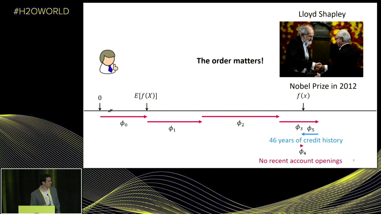
I'm literally filling out that form for John. And then I observed the change that was made in the model. Okay. So I set the application to say, your income's not verified, and then I simply let all the rest of the stuff be averaged out. Okay. And I note that everything moves out by 2.2%. Now, if I continue doing this and I introduce the debt to income ratio, I see that it's at 30, which if you've seen a lot of debt to income ratios, that's rather high, and this pushes the risk all the way up to 21%. And then we see that he was delinquent on payment 10 months ago, this is not good news for John. But he hasn't applied for any recent account openings, so that's good, drops his risk way down cause apparently he's not applying for credit recently. But he has 46 years of credit history. So that apparently is bad for him and jumps him up to our final outcome. Now, why is this the final outcome? Because I trained a model with only five variables to make a nice clean slide. Okay. Of course, we do this in the real world, you're gonna end up with hundreds of these things. But typically only a few of them are really impactful for any individual.
So are we done, right? I just showed you a way to just literally fill out the form one at a time and measure the Delta as I put each value into his application, and then we can consider ourselves done. But of course, we're not, because this is not a simple linear model, potentially could be a very complex model. And so the order here really matters. So no recent account openings, for example, in 46 years of credit history, it could be that maybe no recent account, it kinda looks like 46 years is almost sort of undoing your recent account openings, right? Like maybe it's that it's not important to have no recent account openings if you have a long credit history. I don't know, could be true. So we could test that by swapping the order in which we introduce these features, we could introduce credit history first, and then we could introduce his account openings, just filling out his application in a different order.
It turns out that if we do that, we get totally different attributions given to these features. Indeed 46 years of credit history actually now helps him a little bit. And then no recent account openings are just meaningless, given the fact that we knew his long credit history. So, you know, this is an actual model that was trained on actual data. This is to highlight the fact that strong interaction effects can exist and you can't just pick a particular order and think that you've solved it. So what do we do here? Well, this is kind of where it's good to step back and ask if people have asked about this problem, you know, kind of tackled this issue before. And it turns out that they have, back in game theory in the 1950s, they were working on fairly allocating credit among players in a game, where fairness was written down according to some axioms.
Shapley Values
And it turns out that just like you would want to fairly allocate credit for the outcome of a game to collaborating players who may have contributed unequally, so also you would like to fairly allocate credit to features as they come into a model and potentially contribute unequally to the output of that model. So this was brought together by Lloyd Shapley, and he did a lot of great work on this and got him a fancy prize. And one of the proposals that he did in his work is how to allocate credit for these games. And his proposal became known as the Shapley Values. Okay. So that's where its name comes from. And what are these axioms of fairness, cause that's really important here? I'm gonna go all these pretty quickly, but essentially they mean two things. There are two really important axioms that need to be kept in mind here.
One is that I would like my credit to sum up from the expected value of my model's output to the actual output for my current example. So this basically just says, I want these things to sum up. I would like my credit to be fully allocated, none extra, none left over. So this seems like a natural one, it helps the interpretation of these things. The second one is a little bit more complicated, but even more important, and that is if I have two models and one of them features two has a bigger red bar than the other model, no matter what order I pick, that means that that feature is certainly more important in that model. Okay. In all situations that feature always makes a bigger difference in one model than another, then I certainly shouldn't give the model with the less impact more credit. That's essentially what Monotonicity says.
So if this doesn't hold, then you really can't trust future orderings. So this is a really critical one. So given these two things, you know, Shapley showed that there's this unique allocation approach. And given that we're working with this sort of filling out the application one at a time view of the world, we now have a unique answer. We have these Shapley Values. The problem, of course, is that they're really easy to state, here's the data scientist like, great you sold me, how do I compute these? I said that's really easy. You just do what I just told you. You just do it in factorial times where N is the number of features. Of course, if you're a data scientist and you know math, you kind of glaze over at that point. Turns out this is particularly hard if you're in computer science, which means you'll be famous if you solve it.
And so on this part, I'm gonna skip over a lot of the math details, because this is actually where most of our core contribution comes in. You know, a lot of the stuff that I described before has been discussed in literature before, but what we did is work on how we could make this very efficient and write down exact algorithms for this. And it turns out you can solve them very efficiently for specific classes of models, in particular tree-based models we have some nice implementations for. So anything that involves a random forest or a decision tree or if there are any boosted trees, this is a great way to allocate credit.
So let's see how this would work. So let's imagine we now have that fast algorithm. Okay. We're gonna call a package that we have called Shap, which should be very concrete to understand how this works. We're just gonna pass our model to an explainer. We're gonna explain every example in a data set and get a matrix that's the same size as the data matrix we passed in. And then we're gonna start plotting this thing to see what happened. Okay. If we're gonna pass the base rate of our model in, we're gonna pass in the row that corresponds to the explanation for John and we're gonna pass in the row of data that is John's application data. And when we do that we can plot, sort of a nifty little plot like this, where all the red features are kind of pushing the risk higher and the blue features pushing it lower.
So this is the same plot that we saw before, but now these are the actual Shapley Values. So they're kind of guaranteed to have these consistencies. And this is where we get into the debugging part because if you're a data scientist and you look at this, you realize that man 46 years of credit history actually really does actually increase his risk. Okay. And you might kind of ask like, why on earth would your repayment problems go up because you have a long credit history, that seems like a kind of counterintuitive, right? And so in order to dig into this a little bit deeper, we could plot more stuff. So first of all, let's plot months of credit history, and just give our whole matrix of explanations and our data matrix. So when we do that, what we're gonna do is we'll get a plot back that has on the X axis, our months of credit history and on the Y axis, we have the output, the impact on the output of the model.
Okay? So this is roughly familiar, similar to a partial dependence plot. If you've used those before and every dot we're gonna plot a scatter plot here, and every dot here is gonna be a person's application. And what you can see is that people will color it with another feature for extra info. But if you see on the far, I guess it's on the far left, you have an early credit history, you know, people with short credit history and they have high risk. That's natural. You begin to see the sloping down, and then if we look to see where John is, he's right here. So he's got about 500, some months of credit history, which is about 45 years, and what we can see is a really interesting change in about 35, 40 years. And this is of course a problem because the model that I've trained is identifying retirement-age individuals based on their long credit histories.
Okay? So this is a lesson on what can happen when you train a very flexible model on a data set and then don't peek under the hood, right? Things can happen where you really need to explain and debug your models. Okay. Now, as we've talked about, there are lots of tools out there for debugging, and this is one of them. This is one of the tools for looking inside your model and understanding what's going on. Because you might find things like this, that of course you would certainly not want to be rolled out in any practical sense or real-world setting.
So what I've talked about is inside model development, these types of feature attritions are useful for debugging and exploration, but I also wanna touch on one other one, and that is model monitoring, cause it's super useful here as well. So in model monitoring, this is a medical example now. We're gonna talk about a model that's designed to predict the duration of a medical procedure at a hospital. So a surgery, some inpatient kind of setting, it's super important for scheduling people, right? So hospitals use this all the time, and then they deploy it. So what we're gonna do is we're gonna train it on one year of data in this university hospital, and then we're going to simulate a deployment by letting it run for three and a half years. And if you've ever deployed a machine learning model, one of the first things you wanna monitor is it's just loss, right?
What is the loss over time? Is it getting worse? Is it somehow decaying? Is something going south? Well, it turns out, if you look at this it just looks kind of random, but we wanted to test and see how well just looking at the loss kind of helps you debug the model. And so we actually put a bug in the model, right? So inside the model, we just flipped the labels of two of the rooms in the hospital just to see kind of what would this show us. And I guess the question is, can you see where that happened? The answer course is no, because there are, you know, hundreds, I think there's actually a thousand features going into this model. So when I flip two of them, that certainly makes a big difference for those features, but it doesn't impact, it gets lost in the noise of just the random kind of back and forth of your model.
So what I just talked about before was explaining the output of the model. So when you're explaining John's prediction, we were explaining the output of the model. How about we explain the loss of the model? Okay. If we explain the loss of the model, we can now decompose, not the output among each of the input features, but the loss among each of the input features. Which will essentially tell you which input features are driving my accuracy or my lack of accuracy on a per sample basis. So now what we can do is plot that over time for each feature. And if we plot that for the feature that we broke, up is bad, and down is good. The question now is, can you find where we introduced the bug? Or equivalently find some algorithm that's gonna detect some change detection for you automatically. So I had to argue that this kind of deconvolution of your loss down into your input features could be an important tool for the product of model monitoring stuff.
It's not just bugs that we introduced by ourselves, even in this sort of clean data set that we got, course it's been, you know, people have already been through this data set to clean it up. So the fact that we find stuff is informative already. Here's a place where the marginal distribution of your statistic might not change. Okay. So what that means is that if you're watching some sort of marginal distributional test, you would not see sort of a spike in your features change, but the meaning of the feature did change. Okay. And so the impact of the model changed. So here we saw transient EMR records. We can see things like long-term trend changes as well. So to wrap up, I just wanted to point out these two things are kind of interesting applications. But just to get you thinking, I wanted to throw out a bunch of applications in my last 20 seconds or so. One is you can actually, instead of regularizing the parameters of your model, you could regularize the explanation of your model.
Additional Applications
Sometimes that's a much easier way to control model behavior is by making statements about its explanation rather than statements about its parameters. In human-AI collaboration, people have used this for customer retention, where you actually provide explanations to the salesperson calling after a churn model is predicted whether they're gonna churn, super helpful as a calling agent, to know why you're calling. Decision support for doctors, human risk oversight for high-risk financial decisions, a lot of interesting regulatory compliance, and scientific discoveries like grouping people by their explanations. So I'll leave it there, but thanks.