Torch is a scalable and efficient deep learning  framework. It offers flexibility and speed to build large scale applications. It also includes a wide range of libraries for developing speech, image, and video-based applications. The basic building block of Torch is called a tensor. All the operations defined in Torch use a tensor.

Ok, let’s get back to the “why”. Why do we need Torch in the first place?

Why Torch?

Torch is undoubtedly one of the most scalable and efficient deep learning libraries out there. It is well known for its speed and flexibility. Here are the two primary reasons for preferring Torch over others.

1. Torch’s backend is developed in C, C++, and CUDA. It is a very powerful and highly optimized framework.
2. Torch supports parallelization. Hence, model training can be done in parallel across multiple GPUs.

What is PyTorch?

PyTorch  is one of the popular deep learning frameworks for building neural networks . It is built on top of Torch. It uses the same backend as the torch. The core set of torch libraries remains the same. In short, PyTorch is a flexible Python interface for Torch.

Case Study: Stock Price Prediction

Let’s look at a typical deep learning use case – stock price prediction. We have prepared a mini tutorial to walk you through the basics. You will learn how to build a deep learning model for predicting stock prices using PyTorch. For this tutorial, we are using this stock price dataset from Kaggle .

Reading and Loading Dataset

import pandas as pd

df = pd.read_csv("prices-split-adjusted.csv", index_col = 0)

We will use EQIX for this tutorial:

import matplotlib.pyplot as plt

df = df[df.symbol == 'EQIX']

plt.plot(df.open.values, color='red', label='open')

plt.plot(df.close.values, color='green', label='close')

plt.plot(df.low.values, color='blue', label='low')

plt.plot(df.high.values, color='black', label='high')

plt.title('stock price')

plt.xlabel('time [days]')

plt.ylabel('price')

plt.legend(loc='best')

Data Normalization

This is an important pre-processing step for neural networks:

import sklearn.preprocessing

min_max_scaler = sklearn.preprocessing.MinMaxScaler()

df['open'] = min_max_scaler.fit_transform(df.open.values.reshape(-1,1))

df['high'] = min_max_scaler.fit_transform(df.high.values.reshape(-1,1))

df['low'] = min_max_scaler.fit_transform(df.low.values.reshape(-1,1))

df['close'] = min_max_scaler.fit_transform(df['close'].values.reshape(-1,1))

data = df[['open','close','low','high']].values

Preparing Data for Time Series

In order to prepare the dataset for stock price prediction, we need to frame it as a time series problem. We will use the price from the previous 19 days to predict the price on the next day. Let’s create the sequences accordingly:

import numpy as np

seq_len=20

sequences=[]

for index in range(len(data) - seq_len): 

 sequences.append(data[index: index + seq_len])

sequences= np.array(sequences)

Splitting the Data

We divide the entire dataset into three parts. 80% for the training set, 10% for the validation set and the remaining 10% for the test set:

valid_set_size_percentage = 10 

test_set_size_percentage = 10 

valid_set_size = int(np.round(valid_set_size_percentage/100*sequences.shape[0])) 

test_set_size = int(np.round(test_set_size_percentage/100*sequences.shape[0]))

train_set_size = sequences.shape[0] - (valid_set_size + test_set_size)

x_train = sequences[:train_set_size,:-1,:]

y_train = sequences[:train_set_size,-1,:]

x_valid = sequences[train_set_size:train_set_size+valid_set_size,:-1,:]

y_valid = sequences[train_set_size:train_set_size+valid_set_size,-1,:]

x_test = sequences[train_set_size+valid_set_size:,:-1,:]

y_test = sequences[train_set_size+valid_set_size:,-1,:]

Creating Data Loaders

Next, we define the data loaders to load the dataset in batches:

import torch

from torch.utils.data import TensorDataset, DataLoader

x_train = torch.tensor(x_train).float()

y_train = torch.tensor(y_train).float()

x_valid = torch.tensor(x_valid).float()

y_valid = torch.tensor(y_valid).float()

train_dataset = TensorDataset(x_train,y_train)

train_dataloader = DataLoader(train_dataset, batch_size=32, shuffle=True)

valid_dataset = TensorDataset(x_valid,y_valid)

valid_dataloader = DataLoader(valid_dataset, batch_size=32, shuffle=True)

Defining Model Architecture

We will define the model architecture by subclassing the nn (Neural Networks) module. As it’s a time series problem, we will use Long Short-term Memory (LSTM) to capture the sequential information:

from torch import nn

class NeuralNetwork(nn.Module):

 def __init__(self):

 super(NeuralNetwork, self).__init__()

 self.lstm = nn.LSTM(4,64,batch_first=True)

 self.fc = nn.Linear(64,4)

 def forward(self, x):

 output, (hidden, cell) = self.lstm(x)

 x = self.fc(hidden)

 return x

model = NeuralNetwork()

#push to cuda if available

device = torch.device('cuda' if torch.cuda.is_available() else 'cpu') 

model = model.to(device)

We also need to define the optimizer and loss:

import torch.optim as optim

optimizer = optim.Adam(model.parameters())

mse = nn.MSELoss()

Model Training

First, we define the forward and backward pass for training the neural network:

def train(dataloader):

 epoch_loss = 0

 model.train() 

 for batch in dataloader:

 optimizer.zero_grad() 

 x,y= batch

 pred = model(x)

 loss = mse(pred[0],y) 

 loss.backward() 

 optimizer.step() 

 epoch_loss += loss.item() 

 return epoch_loss

Now, let us define only the forward pass for evaluating the model performance:

def evaluate(dataloader):

 epoch_loss = 0

 model.eval() 

 with torch.no_grad():

 for batch in dataloader: 

 x,y= batch

 pred = model(x)

 loss = mse(pred[0],y) 

 epoch_loss += loss.item() 

 return epoch_loss / len(dataloader)

Let’s train the model for 50 epochs. We will also save the best model during training based on the validation loss.

n_epochs = 50

best_valid_loss = float('inf')

for epoch in range(n_epochs):

 train_loss = train(train_dataloader)

 valid_loss = evaluate(valid_dataloader)

 #save the best model

 if valid_loss < best_valid_loss:

 best_valid_loss = valid_loss

 torch.save(model, 'saved_weights.pt')

 print("Epoch ",epoch+1)

 print(f'\tTrain Loss: {train_loss:.5f}')

 print(f'\tVal Loss: {valid_loss:.5f}\n')

You can expect to see output like this:

Epoch 1

Train Loss: 1.43529

Val Loss: 0.00513

Epoch 2

Train Loss: 0.04183

Val Loss: 0.00080

...

Epoch 49

Train Loss: 0.00499

Val Loss: 0.00041

Epoch 50

Train Loss: 0.00501

Val Loss: 0.00042

Model Inference

We are ready to make some predictions. First, we load the best model:

model=torch.load('saved_weights.pt')

Let’s make predictions on the test set:

x_test= torch.tensor(x_test).float()

with torch.no_grad():

 y_test_pred = model(x_test)

y_test_pred = y_test_pred.numpy()[0]

Finally, we visualize the predictions and compare them with the ground truth:

idx=0

plt.plot(np.arange(y_train.shape[0], y_train.shape[0]+y_test.shape[0]),

 y_test[:,idx], color='black', label='test target')

plt.plot(np.arange(y_train.shape[0], y_train.shape[0]+y_test_pred.shape[0]),

 y_test_pred[:,idx], color='green', label='test prediction')

plt.title('future stock prices')

plt.xlabel('time [days]')

plt.ylabel('normalized price')

plt.legend(loc='best')

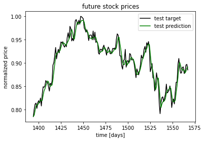
There you have it. We have built a simple neural networks model for stock price prediction using PyTorch. The code complexity tends to increase when you need to build more complex models and fine-tune model architecture for better accuracy.

So the big question is, can we simplify the process and lower the barrier to entry?

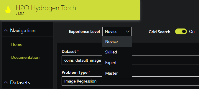
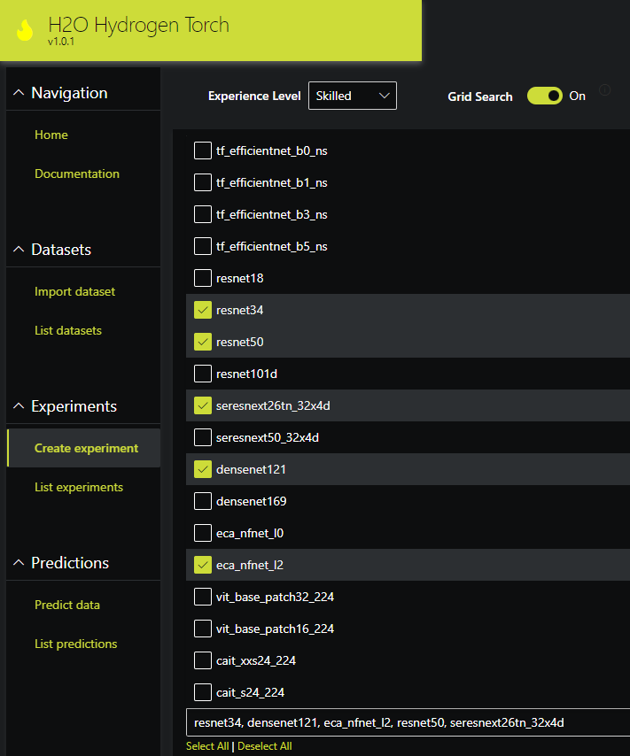
Deep Learning Frameworks Made Simple

That is the question we keep asking ourselves at H2O. In order to democratize deep learning, we have:

• Added support for PyTorch to Driverless AI (see our documentation here).
• Released H2O Hydrogen Torch – a no-code deep learning framework last week (check out our blog post).

H2O Hydrogen Torch – Choose Your Experience Level from Novice (Basic Model Configuration) to Master (Tweak Everything!)

H2O Hydrogen Torch – Enable Grid Search to Find the Optimal Model Architecture

You can get hands-on experience with all these tools right now on H2O AI Cloud . Just sign up for a free demo today.