In a previous article [1], we discussed how machine learning could be harnessed to mitigate fraud. This time, we’ll delve into a step-by-step guide on leveraging H2O AI Cloud to construct efficient fraud detection models. We’ll tackle this process in three critical stages: build, operate, and detect. First, we’ll utilize Driverless AI in H2O AI Cloud to construct the models. The model is constructed using advanced methods, and its interpretability is ensured through Shapley’s Explanations and other methods that are crucial in the context of financial settings.

In the deployment phase, we operationalize the model using H2O MLOps, offering an array of deployment options, including REST API and several programming languages. Once deployed, the model endpoint can be integrated into any downstream application for real-time fraud detection. The model’s continuous performance is evaluated and adjusted according to business KPIs and model performance metrics via a specialized Diagnostics approach. This setup enables a cost-efficient and effective approach to fraud detection that can be dynamically tuned based on real-world experience and changing conditions.

Phase 1: Build

In this initial phase, our aim is to construct a supervised machine-learning model. We’ll start by feeding Driverless AI with a labeled dataset — a set of past transactions that have been reviewed and tagged by fraud analysts as either fraudulent or legitimate. Driverless AI will then learn from this data, developing a keen understanding of what “normal” transaction behavior looks like. This helps the model flag any transactions that diverge from this norm — potential fraud.

Incorporating methods like random forest, gradient boosting, or deep learning, the model will be able to detect intricate patterns and relationships in the data. These techniques empower our model to catch fraud patterns that could potentially be missed by simpler models or rules-based systems. I strongly recommend revisiting our previous article for a more in-depth understanding of the limitations inherent in rule-based systems and the reasoning behind the adoption of machine learning, particularly the AutoML approach.

Dataset

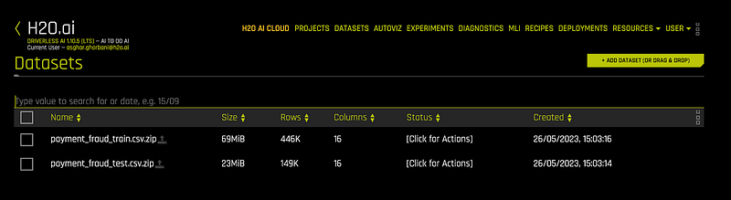
The dataset utilized in this case study is based on BankSim [2], a bank payments simulator for fraud detection research. BankSim generates synthetic data which imitates real-world banking transactions, enabling meaningful research into fraud detection. Our study’s dataset encompasses approximately half a million entries, partitioned into an 80% training and 20% testing dataset. We’ll let Driverless AI dictate the validation split strategy, including whether to use cross-validation or other methods.

The images provided below display a screenshot from the datasets page in Driverless AI, showcasing the row count and a summary of the dataset.

 

EDA — Automatic Visualisation

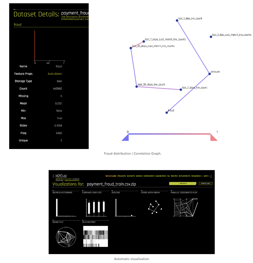
Driverless AI automates the generation of a visualization dashboard based on the dataset, significantly aiding the Exploratory Data Analysis (EDA) process. By auto-generating graphs relevant to the specific dataset, it not only accelerates the EDA process but also draws attention to the most vital dataset information.

The following diagram presents sample graphs in Driverless AI. For instance, these graphs indicate a correlation between the last day’s transactions and the transaction amount and, subsequently, a correlation between the transaction amount and fraud.

However, as can be seen, the fraud column in our dataset is significantly imbalanced, a phenomenon we anticipated. Notably, fraudulent transactions constitute only about 1% of this dataset.

Model Training

With Driverless AI, model training is a rather straightforward process. You simply select the training dataset and hit “PREDICT.” From there, you specify the target column and the test set [3], as can be seen in the screenshot below.

 

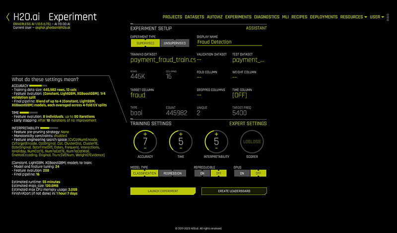
By hitting “LAUNCH EXPERIMENT,” Driverless AI then initiates the model-building process, performing data sanity checks, feature engineering, model building, hyperparameter tuning, and model selection, all automatically via a genetic algorithm.

Despite being an AutoML system, Driverless AI allows expert data scientists significant flexibility. Under the expert settings, they can adjust experiment-related settings, such as feature engineering and selection, model tuning, and algorithm parameters. Moreover, all these steps can also be executed through Python SDK, allowing users to manage their workflow through interfaces like Jupyter Notebook.

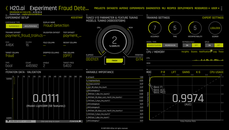
The screenshot below provides an example of an ongoing experiment. As an experiment runs, you can monitor what algorithms are being used, the variables contributing most to model accuracy, and model performance in real time. If you spot an aspect of the modeling that needs alteration, you can stop and adjust the experiment immediately.

 

Once the experiment is complete, you can:

• Interpret the final model.
• Download automatically generated, human-readable documentation of the experiment in MS Word or Markdown format, also known as AutoDoc.
• Download the prediction results on the training, validation, and test data.
• Deploy the model or download the scoring pipeline to run the model inside a custom scoring pipeline.

Machine Learning Interpretation and Transparency

In regulated industries like finance and insurance, the transparency of the model is crucial. Here, we’ll highlight a few key aspects.

One of the first things we look at in an experiment is the model’s interpretations. Driverless AI provides robust interpretability of machine learning models to explain modeling results in a format that is comprehensible to humans. In the Machine Learning Interpretability (MLI) view, Driverless AI employs a host of different techniques and methodologies for interpreting and explaining the results of its models. A number of charts are generated automatically (depending on experiment type), including K-LIME, Shapley, Variable Importance, Decision Tree Surrogate, Partial Dependence, Individual Conditional Expectation, Sensitivity Analysis, NLP Tokens, NLP LOCO, and more. Additionally, you can download a CSV of LIME, Shapley, and Original (Kernel SHAP) Shapley reason codes, as well as text and Python files of Decision Tree Surrogate model rules from this view. The techniques and methodologies used by Driverless AI for model interpretation can be extended with recipes (Python code snippets).

In this article, we’ll briefly discuss Shapley values and Decision Tree Surrogate rules. For a more detailed explanation of other techniques, please refer to the documentation page: https://docs.h2o.ai/driverless-ai/1-10-lts/docs/userguide/interpreting.html

Shapley Explanations

Shapley explanations offer a unified and consistent approach to attribute the contribution of each feature to the prediction made by the model. This technique originated from cooperative game theory and was named after Lloyd Shapley, the Nobel laureate who formulated it. One of the primary advantages of Shapley values is that they always sum up to the total prediction for the model, ensuring a fully accountable allocation of contributions.

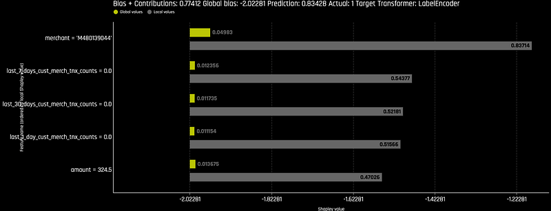
Local Shapley values are calculated by tracing single rows of data through a trained tree ensemble and aggregating the contribution of each input variable as the row of data moves through the trained ensemble. This makes it possible to see how much each feature contributes to a specific prediction. In our case, if the prediction is a fraud, we then can use Shapley values to highlight the important input features that lead the model to believe the transaction is fraudulent. This increases transparency as it explains why the model made a specific prediction, boosting confidence in the model’s outcome and aiding fraud analysts to expedite the review process if a transaction is sent for a review.

In Driverless AI, the Shapley values for each feature in a prediction can be easily accessed and used to drive understanding and interpretability. This way, we can answer questions like why a specific transaction has been flagged as fraudulent. For instance, in a plot showing the Shapley values for a fraudulent transaction, among the top most influential factors, we see the merchant id and the transaction amount. This means that these two features strongly contribute to the model’s decision that a given transaction is likely fraudulent.

By providing a measure of how each feature contributes to the decision-making process of the model, Shapley explanations enable a better understanding of the model, improving its transparency and trustworthiness. They can be especially useful in regulated industries where the interpretability and fairness of machine learning models are of paramount importance.

 

These values also can be available at the prediction time through the APIs and can be integrated into any downstream applications.

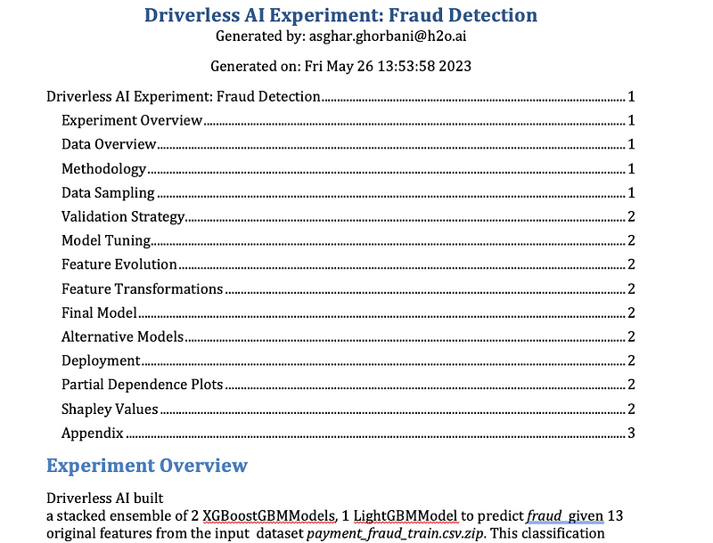
AutoDoc

AutoDoc is an essential tool for reviewing the model as part of the model approval process. It generates automatic machine-learning documentation for individual Driverless AI experiments. This editable document includes an overview of the experiment and other important details like feature engineering, model selection and tuning, model evaluation, and final model performance. Refer below to see an example of content on what to expect from exporting such automated documentation.

 

Phase 2: Deployment and Productionization

Now that we’ve built and assessed our model using machine learning interpretability and we’re confident in its performance, it’s time to deploy it using H2O MLOps. H2O MLOps is a flexible, open platform geared toward model deployment, management, governance, and monitoring. It is seamlessly integrated with Driverless AI. The steps below will guide you in creating H2O MLOps deployments directly from the completed experiment page in Driverless AI.

1. Navigate to the completed experiment page and click on the “Deploy” button.
2. Next, click the H2O MLOps button. Depending on how your experiment is organized, one of the following scenarios will occur:
3. If the experiment is linked to a single Project, you’ll be redirected to that Project’s detail page in the H2O MLOps app.
4. If the experiment is linked to multiple Projects, choose the Project you wish to navigate to in the H2O MLOps app. Alternatively, you can create a new Project to assign the experiment to. If you opt for a new Project, you’ll be prompted to provide a name and description. After setting up the new Project and associating it with the experiment, click the “Go to MLOps page” button to navigate to your Project’s detail page in the H2O MLOps app.
5. If the experiment isn’t assigned to any Project, choose an existing Project to link it to, or create a new Project and link the experiment to that.
6. Next, on the project page (within the MLOps) in the Experiments tab, select the experiment and register it either as a new model or as a new version of an existing model.
7. Following this, you’re ready to deploy the model. In the Deployments tab, click on “Create Deployment” and follow the instructions. Here, you have several options: you can deploy a single model, use A/B testing, or use the challenger/Champion model. Your choice will depend on your specific needs.
8. In the advanced settings, you have the option to configure a unique endpoint path.
9. Furthermore, you can specify the runtime, where you have the choice of whether the endpoint exposes the Shapley values.
10. Once the model is successfully deployed and is in a healthy state, click on the model name. You will then be able to copy the endpoint and incorporate it into any downstream application. You can also see a sample endpoint call on that page.

Additional Deployment Options

By default, each completed Driverless AI experiment generates at least one scoring pipeline for Python, C++, Java, and R. Hence, you have an array of deployment options for Driverless AI MOJO (Java and C++ with Python/R wrappers) and Python Scoring pipelines for production. If the REST API (as discussed above) does not meet your requirements, you can download and run any of the artifacts in your preferred runtime environment. In this article, however, we have focused on MLOps deployment via the REST API.

Phase 3: Fraud Detection Application

Congratulations on reaching this stage! You now have access to a fraud detection model endpoint that’s ready to help identify fraudulent transactions. This endpoint, discussed in the previous section, can be integrated into any application capable of interacting with a REST API.

As part of this project, I’ve utilized the H2O Wave framework for prototyping an application that interacts with our model endpoint swiftly. This application can send transaction details to the endpoint and receive back predictions indicating whether the transaction is likely fraudulent. It also retrieves Shapley values, allowing us to understand which input features are contributing most significantly to a fraud prediction. You can learn more about the Wave framework on their website: https://wave.h2o.ai/

We have a prototype of this application available for trial. Don’t hesitate to get in touch if you’d like to explore its capabilities further.

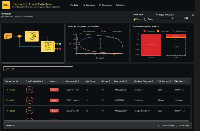
If you’re using our cloud environment, you can easily find this application. Just navigate to the app store and search for the “Transaction Fraud Detection” app. Clicking on the app’s icon will take you to its page, where you can launch the app with a simple click on “run.”

Once launched, you’ll land on the app’s homepage, where you’ll find several key details:

• Model type: This could be single or mixed. In this article, we’ve focused on a single-model approach. A future article will explore the hybrid model, which combines the supervised approach (as discussed above) with an unsupervised (anomaly detection) approach.
• Model Net Loss and Recovery for various thresholds.
• The model’s impact on savings, considering the reduction in false positives and fraud prevention.
• A list of transactions already scored by the model.

This application offers a comprehensive suite of tools for an enhanced understanding of transaction fraud detection.

 

Before proceeding further, I’d like to underscore a few key points concerning the model evaluation within a business setting, with a particular focus on classification models. A classification model, like the one we have built, works by predicting the likelihood of an event occurring. It essentially provides us with a probability rather than a definite yes or no. For instance, if we’re aiming to detect fraudulent transactions, our model might estimate the probability of a given transaction being fraudulent. But to convert this probability into an actionable decision, we need to set a threshold. This threshold acts as our benchmark or criterion to categorize a transaction as fraudulent (a “positive” case) or not. For example, if the probability exceeds 0.4 (or any other predetermined value), we would classify the transaction as fraudulent. If it falls below this threshold, we would consider it legitimate.

However, it’s important to acknowledge that no model can predict with perfect accuracy. We will always encounter two types of errors in our predictions — false positives and false negatives. False positives occur when our model inaccurately flags a legitimate transaction as fraudulent. On the other hand, false negatives happen when fraudulent transactions slip through undetected. Both these errors can have different impacts on our operations, and we need to be mindful of them when setting our threshold.

This is where balancing comes into play. The trick lies in adjusting the threshold so that we can manage these two types of errors in a way that best suits our needs and maximizes business KPIs. It’s about finding the optimal compromise between false positives and false negatives that aligns with our business objectives.

Every business situation is unique, and the ideal balance might be different depending on the specific costs associated with each type of error. In our case, we are considering the cost implications of each error type based on transaction amounts and potential business loss:

• For false negatives, where fraudulent transactions go undetected, we associate this with the transaction amount as it represents a direct loss to the business.
• For false positives, where we mistakenly identify legitimate transactions as fraudulent, we assume certain costs associated with the review process, business interruptions, and potential loss of business.

Loss Gains Analysis

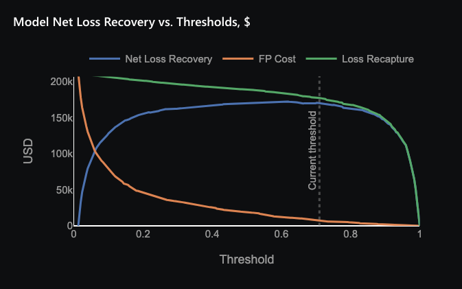
Based on the assumption above, we’ve generated a plot comparing the cost of false positives and the gains from preventing false negatives (“loss recapture”) against our probability threshold. Additionally, this plot shows the “net loss recovery,” the combined impact of these two factors. Our goal is to maximize this net loss recovery, balancing the costs and benefits.

The plot indicates that the optimal threshold is 0.7. At this threshold, our model best balances the costs of false positives and the gains from preventing false negatives, maximizing our net loss recovery. However, due to the dynamic nature of fraud detection, it’s essential to periodically reassess this threshold with a new dataset and potentially a new model.

 

The plot below illustrates the savings achieved by utilizing the model for fraud detection and applying the previously mentioned threshold of 0.7.

 

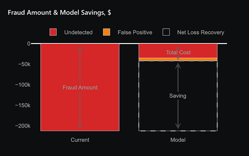
The bar chart presents a comparison between the total cost of fraud before and after the deployment of our model. The left bar represents the total cost of fraud without the model, while the right bar breaks down the costs after the model’s implementation.

In the right bar, the red section indicates fraud instances that still go undetected due to the model’s inherent limitations. The orange section represents additional costs associated with false positives, which require further verification and review. The total height of the right bar represents the combined cost of undetected fraud and false positive instances after deploying the model.

The difference between the left and right bars signifies the savings achieved through the model’s deployment. These substantial savings underscores the model’s effectiveness in reducing the overall costs related to fraud.

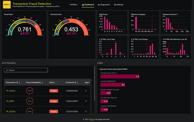
Individual Prediction Dashboard

Next, we would like to look at a dashboard for individual transactions and model prediction. The dashboard screenshot you’re viewing below provides a detailed breakdown of an individual transaction, predicted as fraudulent, with a probability of 0.76. The first graph on the top left shows the probability of fraud for this transaction, categorizing it as potentially fraudulent based on our set threshold (0.7).

The following six graphs on the top right display the value distribution of various input features across the entire dataset. These can provide valuable context, allowing us to compare the specific values of these features for this transaction against their overall distribution in our portfolio.

Lastly, the dashboard includes a chart, bottom right, that highlights the crucial factors contributing to this fraud prediction. In this instance, it’s observed that the payment amount and the merchant are the most influential factors driving the high fraud probability. This insight can aid fraud analysts in understanding the model’s decision and in making their subsequent review more effective. This dashboard, thus, offers an in-depth understanding of individual transactions, their comparison with the broader portfolio, and the key factors influencing their classification, enhancing our fraud detection capabilities.

 

Diagnostics

The Diagnostics page in our application is designed to facilitate the ongoing evaluation of the model using a test dataset. For instance, after the model has been in use for some time, we might gather a new set of data reflecting transactions that have been confirmed as fraudulent or legitimate, perhaps following a review process.

This Diagnostics page is instrumental in fine-tuning the threshold based on various parameters. These parameters might include standard model performance metrics such as accuracy and the F1 score, as well as business KPIs such as cost savings, which we’ve discussed earlier.

When you upload the new test dataset, the system can optimize the threshold accordingly. This update allows you to review a fresh confusion matrix, a table that presents a summary of the model’s performance. More crucially, it includes a cost-sensitive confusion matrix that considers the actual business costs and benefits of different outcomes.

 

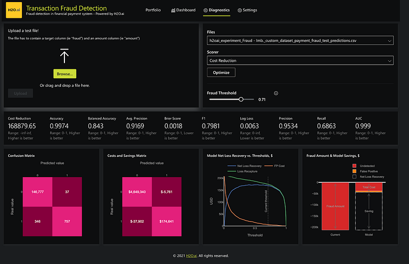
This page, in essence, enables you to refine the model based on real-world experience and changing conditions, ensuring that our fraud detection efforts remain as effective and cost-efficient as possible.

Conclusion

In conclusion, the use of machine learning and AI for fraud detection has undeniably transformative potential for businesses across various sectors. The H2O AI Cloud’s platform embodies this promise by providing a comprehensive and accessible framework for model building, deployment, and business application. The Shapley Explanations offer invaluable insight, ensuring interpretability and confidence in AI-driven decisions. As the adoption of AI becomes an increasingly strategic imperative for enterprises, we at H2O.ai stand ready to support your journey and address the unique challenges of your organization with our robust, user-friendly, and adaptable AI platform.

References

- Reducing False Positives in Financial Transactions with AutoML /en/blog/2023/reducing-false-positives-in-financial-transactions-with-automl
- Lopez-Rojas, Edgar Alonso, and Stefan Axelsson. “Banksim: A bank payments simulator for fraud detection research.” 26th European Modeling and Simulation Symposium, EMSS. 2014.
- The test set is not mandatory, and if present, it serves as a holdout set. This implies that it won’t be utilized in any way for optimization or model selection during the modeling process.