Creating and plotting decision trees (like one below) for the models created in H2O will be the main objective of this post:

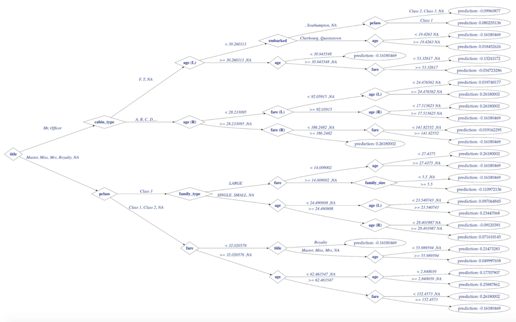
Figure 1. Decision Tree Visualization in R

Decision Trees with H2O

With release 3.22.0.1 H2O-3 (a.k.a. open source H2O or simply H2O) added to its family of tree-based algorithms (which already included DRF, GBM, and XGBoost) support for one more: Isolation Forest (random forest for unsupervised anomaly detection). There was no simple way to visualize model trees until recently except following clunky (albeit reliable) method of creating a MOJO object and running a combination of Java and dot commands.

That changed in 3.22.0.1 too with the introduction of unified Tree API to work with any of the tree-based algorithms above. Data scientists are now able to utilize powerful visualization tools in R (or Python) without resorting to producing intermediate artifacts like MOJO and running external utilities. Please read this article by Pavel Pscheidl who did a superb job of explaining H2O Tree API and S4 classes in R before coming back to take it a step further to visualize trees.

The Workflow: from Data to Decision Tree

Whether you are still here or came back after reading Pavel’s excellent post let’s set goal straight: create single decision tree model in H2O and visualize its tree graph. With H2O there is always a choice between using Python or R – the choice for R here will become clear when discussing its graphical and analytical capabilities later.

CART models operate on labeled data (classification and regression) and offer arguably unmatched model interpretability by means of analyzing a tree graph. In data science there is never single way to solve given problem so let’s define end-to-end logical workflow from “raw” data to visualized decision tree:

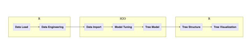
Figure 2. Workflow of tasks in this post

One may argue that the choice of executing steps inside H2O or R could be different but let’s follow the outlined plan for this post. Next diagram adds implementation details:

• R package data.table for data munging
• H2O grid for hyper-parameter search
• H2O GBM for modeling single decision tree algorithm
• H2O Tree API for tree model representation
• R package data.tree for visualization
   

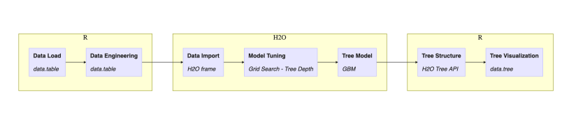
Figure 3. Workflow of tasks in this post with implementation details

Discussion of this workflow continues for the rest of this post.

Titanic Dataset

The famous Titanic dataset contains information about the fate of passengers of the RMS Titanic that sank after colliding with an iceberg. It regularly serves as toy data for blog exercises like this.

H2O public S3 bucket holds the Titanic dataset readily available and using package data.table makes it fast one-liner to load into R:

library(data.table)
titanicDT = fread("https://s3.amazonaws.com/h2o-public-test-data/smalldata/gbm_test/titanic.csv")

Data Engineering

Passenger features from the Titanic dataset are discussed at length online, e.g. see Predicting the Survival of Titanic Passengers and Predicting Titanic Survival using Five Algorithms. To summarize the following features were selected and engineered for decision tree model:

• survived indicates if passenger survived the wreck
• boat and body leak survival outcome and were dropped completely before modeling
• name and cabin are too noisy as they are and only used to derive new features
• title is parsed from name
• cabin_type is parsed from cabin
• family_size and family_type are derived from combination of count features sibsp (siblings+spouse) and parch (parents+children)
• ticket and home.dest are dropped to preserve simplicity of the model
• missing values in age and fare are imputed using target encoding (mean) over grouping by survived, sex, and embarked columns.

Data load and data munging steps above are implemented in R using data.table:

# Titles mapping
TITLES = data.frame(
from=c("Capt", "Col", "Major", "Jonkheer",
"Don", "Sir", "Dr", "Rev", "the Countess",
"Mme", "Mlle", "Ms", "Mr", "Mrs", "Miss", "Master", "Lady"),
to = c("Officer", "Officer", "Officer", "Royalty", "Royalty",
"Royalty", "Officer", "Officer", "Royalty",
"Mrs", "Miss", "Mrs", "Mr", "Mrs", "Miss", "Master", "Royalty"),
stringsAsFactors = FALSE)

# Create features
titanicDT[,
c("sex", "embarked", "survived", "pclass", "cabin_type",
"family_size", "family_type","title") :=
list(
factor(sex, labels = c("Female","Male")),
factor(embarked, labels = c("", "Cherbourg",
"Queenstown","Southampton")),
factor(-survived, labels = c('Yes','No')),
factor(pclass, labels = c("Class 1","Class 2","Class 3")),
as.factor(substring(cabin, 1, 1)),
sibsp + parch,
as.factor(ifelse(sibsp + parch <= 1, "SINGLE",
ifelse(sibsp + parch <= 3, "SMALL", "LARGE"))),
as.factor(sapply(strsplit(name, "[\\., ]+"), function(x) {
words = trimws(x)
words = words[!words=="" ]
words = words[words %in% TITLES$from]
if (length(words) > 0)
title_word = words[[1]]
else
return(NA)
return(TITLES[title_word == TITLES$from, 'to'])
}))
)]

# Handle missing values by imputing them with nulls
titanicDT[, c("age","fare") :=
list(ifelse(is.na(age), mean(age, na.rm=T), age),
ifelse(is.na(fare), mean(fare, na.rm=T), fare)),
by = c("survived","sex","embarked")]

# create dataset for Titanic survived predictive model
response = "survived"
predictors = setdiff(
colnames(titanicDT),
c(response,"name","ticket","cabin","boat","body","home.dest"))

titanicDT = titanicDT[, c(response, predictors), with=FALSE]

Starting with H2O

Creating models with H2O requires running a server process (remote or local) and a client (package h2o in R available from CRAN) where the latter connects and sends commands to the former. The Tree API was introduced with release 3.22.0.1 (10/26/2018) but due to CRAN policies, h2o package usually lags several versions behind (on the time of this writing CRAN hosted version 3.20.0.8). There are two ways to work around this:

1. Install and run package available from CRAN and use strict_version_check=FALSE inside h2o.connect() to communicate with the newer version running on server
2. Or install the latest version of h2o available from H2O repository either to connect to the remote server or to both connect and run server locally.

Tree API is available only with 2D option because it requires access to new classes and functions in h2o package (remember, I asked you to read Pavel’s blog).

Below code from the official H2O download page shows how to download and install the latest version of the package:

# The following two commands remove any previously installed H2O packages for R.
if ("package:h2o" %in% search()) { detach("package:h2o", unload=TRUE) }
if ("h2o" %in% rownames(installed.packages())) { remove.packages("h2o") }

# Next, we download packages that H2O depends on.
pkgs <- c("RCurl","jsonlite")
for (pkg in pkgs) {
if (! (pkg %in% rownames(installed.packages()))) { install.packages(pkg) }
}

# Now we download, install and initialize the H2O package for R.
install.packages("h2o", type="source",
repos="http://h2o-release.s3.amazonaws.com/h2o/rel-xia/2/R")

# Finally, let's load H2O and start up an H2O cluster
library(h2o)
h2o.init()

titanicHex = as.h2o(titanicDT)

Building Decision Tree with H2O

While H2O offers no dedicated single decision tree algorithm there are two approaches using superseding models:

• Distributed Random Forest (DRF) function h2o.randomForest() with arguments
  ntrees = 1
  mtries = number of features (would be determined dynamically at runtime)
  sample_rate = 1
  min_rows = 1
• Gradient Boosting Machine (GBM) function h2o.gbm() with arguments
  ntrees = 1
  min_rows = 1
  sample_rate = 1
  col_sample_rate = 1

Choosing GBM option requires one less line of code (no need to calculate the number of features to set mtries) so it was used for this post. Otherwise, both ways result in the same decision tree with the steps below fully reproducible using h2o.randomForest() instead of h2o.gbm().

Decision Tree Depth

When building single decision tree models maximum tree depth stands as the most important parameter to pick. Shallow trees tend to underfit by failing to capture important relationships in data producing similar trees despite varying training data (error due to high bias). On the other hand, trees grown too deep overfit by reacting to noise and slight changes in data (error due to high variance). Tuning H2O model’s parameter max_depth that limits decision tree depth aims at balancing the effects of bias and variance. In R using H2O to split data and to tune the model, then visualizing results with ggplot to look for right value unfolds like this:

1. split Titanic data into training and validation sets
2. define grid search object with parameter max_depth
3. launch grid search on GBM models and grid object to obtain AUC values (model performance)
4. plot grid model AUC’es vs. max_depth values to determine “inflection point” where AUC growth stops or saturates (see plot below)
5. register tree depth value at inflection point to use in the final model

Code below implements these steps:

# split into train and validation
splits = h2o.splitFrame(data = titanicHex, ratios = .8, seed = 1234)
trainHex = splits[[1]]
validHex = splits[[2]]

# GBM hyperparamters
gbm_params = list(max_depth = seq(2, 10))

# Train and validate a cartesian grid of GBMs
gbm_grid = h2o.grid("gbm", x = predictors, y = response,
grid_id = "gbm_grid_1tree",
training_frame = trainHex,
validation_frame = validHex,
ntrees = 1, min_rows = 1,
sample_rate = 1, col_sample_rate = 1,
learn_rate = .01, seed = 111,
hyper_params = gbm_params)

gbm_gridperf = h2o.getGrid(grid_id = "gbm_grid_1tree",
sort_by = "auc",
decreasing = TRUE)

# Plot grid model AUC vs. max-depth
library(ggplot2)
library(ggthemes)
ggplot(as.data.frame(sapply(gbm_gridperf@summary_table, as.numeric))) +
geom_point(aes(max_depth, auc)) +
geom_line(aes(max_depth, auc, group=1)) +
labs(x="max depth", y="AUC", title="Grid Search for Single Tree Models") +
theme_pander(base_family = 'Palatino', base_size = 12)

and produces chart that points to inflection point for maximum tree depth at 5:

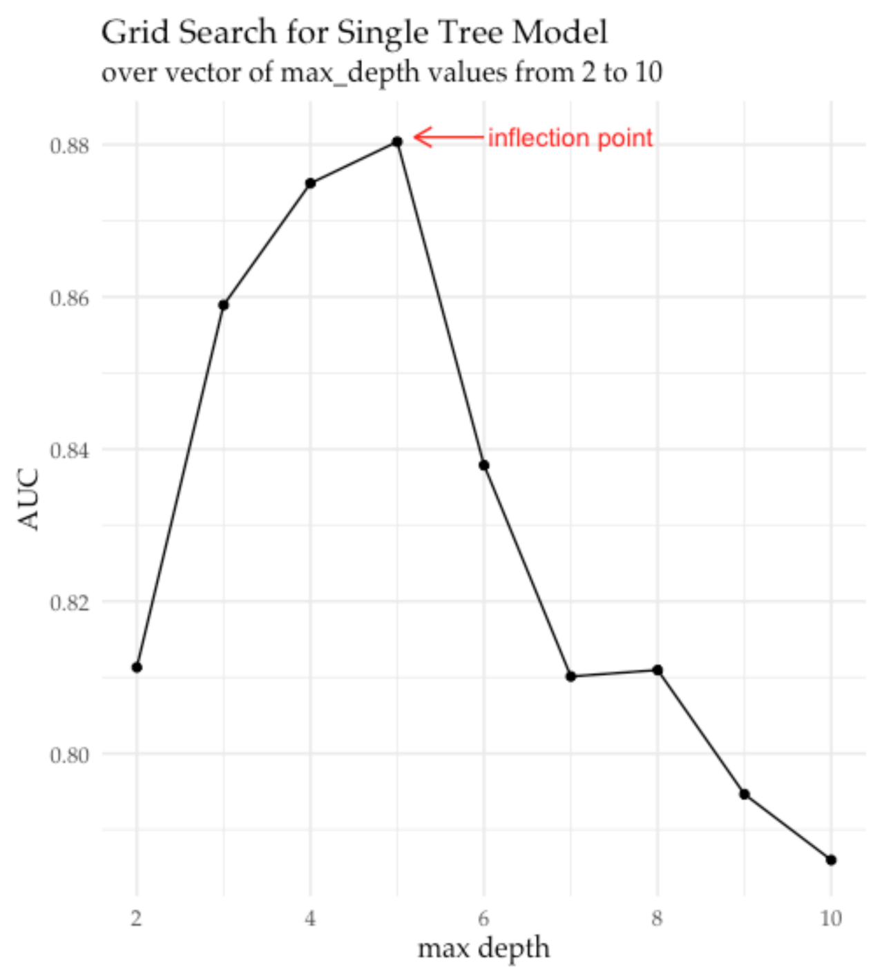
Figure 4. Visualization of AUC vs. maximum tree depth hyper-parameter trend
extracted from the H2O grid object after running grid search in H2O.
Marked inflection point indicates when increasing maximum tree depth
no longer improves model performance on the validation set

Creating Decision Tree

As evident from the Figure 3 optimal decision tree depth is 5. The code below constructs single decision tree model in H2O and then retrieves tree representation from a GBM model with Tree API function h2o.getModelTree(), which creates an instance of S4 class H2OTree and assigns to a variable titanicH2oTree:

titanic_1tree =
h2o.gbm(x = predictors, y = response,
training_frame = titanicHex,
ntrees = 1, min_rows = 1,
sample_rate = 1, col_sample_rate = 1,
max_depth = 5,
# use early stopping once the validation AUC doesn't improve
# by at least 0.01% for 5 consecutive scoring events
stopping_rounds = 3, stopping_tolerance = 0.01,
stopping_metric = "AUC",
seed = 1)

titanicH2oTree = h2o.getModelTree(model = titanic_1tree, tree_number = 1)

At this point, all action moved back inside R with its unparalleled access to analytical and visualization tools. So before navigating and plotting a decision tree – final goal for this post – let’s have a brief intro to networks in R.

Overview of Network Analysis in R

R offers arguably the richest functionality when it comes to analyzing and visualizing network (graph, tree) objects. Before taking on the task of conquering it spend time visiting a couple of comprehensive articles describing the vast landscape of tools and approaches available: Static and dynamic network visualization with R by Katya Ognyanova and Introduction to Network Analysis with R by Jesse Sadler.

To summarize there are two commonly used packages to manage and analyze networks in R: network (part of statnet family) and igraph (family in itself). Each package implements namesake classes to represent network structures so there is significant overlap between the two and they mask each other’s functions. The preferred approach is picking only one of two: it appears that igraph is more common for general-purpose applications while network is preferred for social network and statistical analysis (my subjective assessment). And while researching these packages do not forget about package intergraph that seamlessly transforms objects between network and igraph classes. (And this analysis stopped short of expanding into the universe of R packages hosted on Bioconductor).

When it comes to visualizing networks choices quickly proliferate. Both network and igraph offer graphical functions that use R base plotting system but it doesn’t stop here. Following packages specialize in advanced visualizations for at least one or both of the classes:

• ggraph
• ggnet2
• ggnetwork
• visNetwork
• DiagrammeR
• networkD3

Finally, there is package data.tree designed specifically to create and analyze trees in R. It fits the bill of representing and visualizing decision trees perfectly, so it became a tool of choice for this post. Still, visualizing H2O model trees could be fully reproduced with any of network and visualization packages mentioned above.

Visualizing H2O Trees

In the last step, a decision tree for the model created by GBM moved from H2O cluster memory to H2OTree object in R by means of Tree API. Still, specific to H2O the H2OTree object now contains necessary details about decision tree, but not in the format understood by R packages such as data.tree.

To fill this gap function createDataTree(H2OTree) created that traverses a tree and translates it from H2OTree into data.tree accumulating information about decision tree splits and predictions into the node and edge attributes of a tree:

library(data.tree)

createDataTree <- function(h2oTree) {
h2oTreeRoot = h2oTree@root_node
dataTree = Node$new(h2oTreeRoot@split_feature)
dataTree$type = 'split'
addChildren(dataTree, h2oTreeRoot)
return(dataTree)
}

addChildren <- function(dtree, node) {

if(class(node)[1] != 'H2OSplitNode') return(TRUE)

feature = node@split_feature
id = node@id
na_direction = node@na_direction

if(is.na(node@threshold)) {
leftEdgeLabel = printValues(node@left_levels,
na_direction=='LEFT', 4)
rightEdgeLabel = printValues(node@right_levels,
na_direction=='RIGHT', 4)
}else {
leftEdgeLabel = paste("<", node@threshold,
ifelse(na_direction=='LEFT',',NA',''))
rightEdgeLabel = paste(">=", node@threshold,
ifelse(na_direction=='RIGHT',',NA',''))
}

left_node = node@left_child
right_node = node@right_child

if(class(left_node)[[1]] == 'H2OLeafNode')
leftLabel = paste("prediction:", left_node@prediction)
else
leftLabel = left_node@split_feature

if(class(right_node)[[1]] == 'H2OLeafNode')
rightLabel = paste("prediction:", right_node@prediction)
else
rightLabel = right_node@split_feature

if(leftLabel == rightLabel) {
leftLabel = paste(leftLabel, "(L)")
rightLabel = paste(rightLabel, "(R)")
}

dtreeLeft = dtree$AddChild(leftLabel)
dtreeLeft$edgeLabel = leftEdgeLabel
dtreeLeft$type = ifelse(class(left_node)[1] == 'H2OSplitNode', 'split', 'leaf')

dtreeRight = dtree$AddChild(rightLabel)
dtreeRight$edgeLabel = rightEdgeLabel
dtreeRight$type = ifelse(class(right_node)[1] == 'H2OSplitNode', 'split', 'leaf')

addChildren(dtreeLeft, left_node)
addChildren(dtreeRight, right_node)

return(FALSE)
}

printValues <- function(values, is_na_direction, n=4) {
l = length(values)
if(l == 0)
value_string = ifelse(is_na_direction, "NA", "")
else
value_string = paste0(paste0(values[1:min(n,l)], collapse = ', '),
ifelse(l > n, ",...", ""),
ifelse(is_na_direction, ", NA", ""))
return(value_string)
}

Finally, everything lined up and ready for the final step of plotting decision tree:

• single decision tree model created in H2O
• its structure made available in R
• and translated to specialized data.tree for network analysis.

Styling and plotting data.tree objects is built around rich functionality of the DiagrammerR package. For anything that goes beyond simple plotting read documentation here but also remember that for plotting data.tree takes advantage of:

• hierarchical nature of tree structures
• GraphViz attributes to style graph, node and edge properties
• and dynamic callback functions (in this example GetEdgeLabel(node), GetNodeShape(node), GetFontName(node)) to customize tree’s feel and look

The following code will produce this moderately customized decision tree for our H2O model:

titanicDataTree = createDataTree(titanicH2oTree)

GetEdgeLabel <- function(node) {return (node$edgeLabel)}
GetNodeShape <- function(node) {switch(node$type,
split = "diamond", leaf = "oval")}
GetFontName <- function(node) {switch(node$type,
split = 'Palatino-bold',
leaf = 'Palatino')}
SetEdgeStyle(titanicDataTree, fontname = 'Palatino-italic',
label = GetEdgeLabel, labelfloat = TRUE,
fontsize = "26", fontcolor='royalblue4')
SetNodeStyle(titanicDataTree, fontname = GetFontName, shape = GetNodeShape,
fontsize = "26", fontcolor='royalblue4',
height="0.75", width="1")

SetGraphStyle(titanicDataTree, rankdir = "LR", dpi=70.)

plot(titanicDataTree, output = "graph")

Figure 5. H2O Decision Tree for Titanic Model Visualized with data.tree in R

References

• Anomaly Detection with Isolation Forests using H2O
• Changes in H2O Xia (3.22.0.1) – 10/26/2018
• Visualizing H2O GBM and Random Forest MOJO Model Trees
• Inspecting Decision Trees in H2O
• Classification and Regression Trees
• Predicting the Survival of Titanic Passengers
• Predicting Titanic Survival using Five Algorithms
• Distributed Random Forest (DRF)
• Gradient Boosting Machine (GBM)
• Inflection Point
• Static and dynamic network visualization with R by Katya Ognyanova
• Introduction to Network Analysis with R by Jesse Sadler
• CRAN Graphical Models in R Task View
• Bioconductor GraphAndNetwork packages
• Introduction to data.tree
• DiagrammeR package on github
• Node, Edge, and Graph attributes for Graphviz tools
• Public GitHub gist with source code